Part 1: Shoot the Pictures
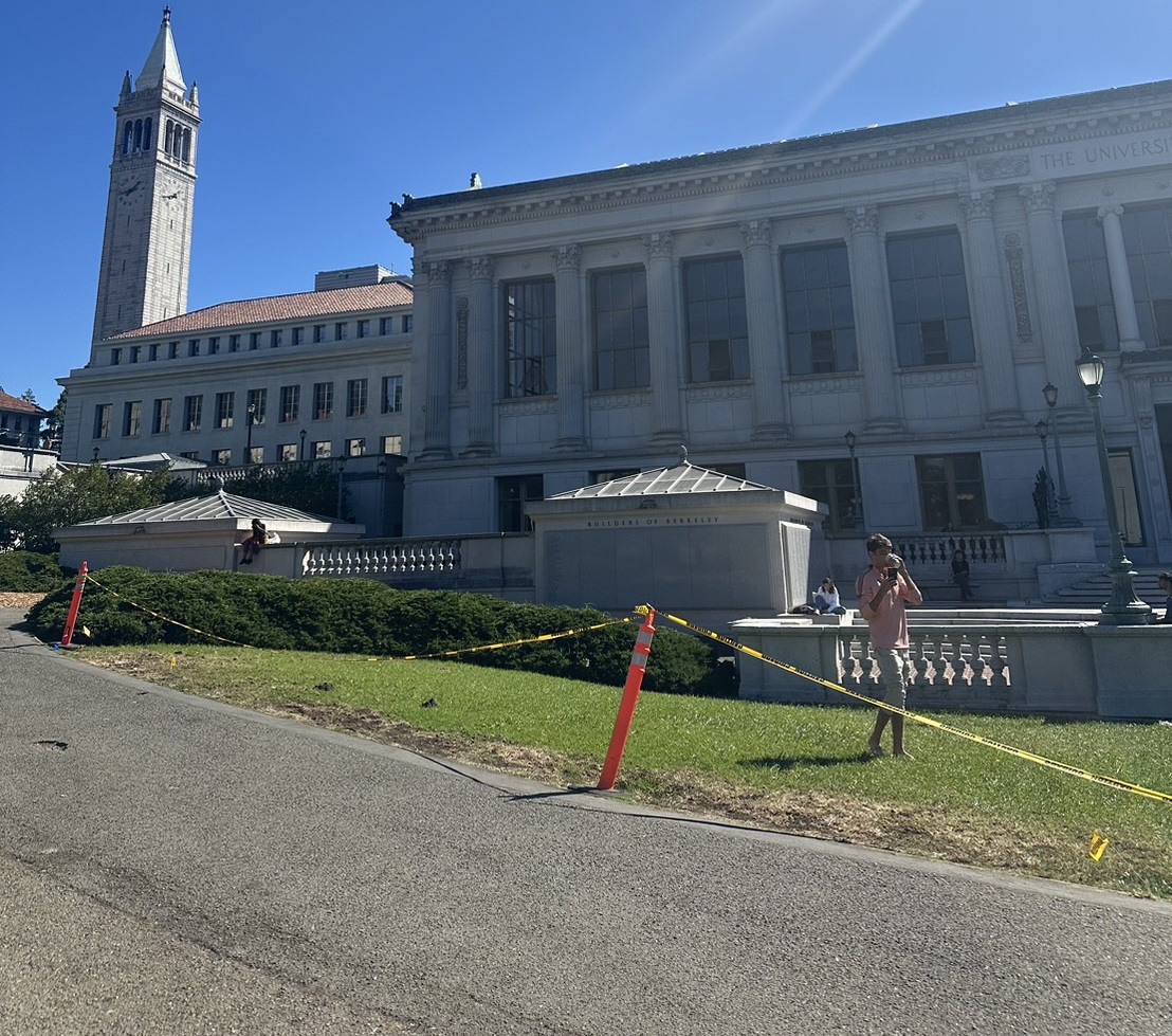
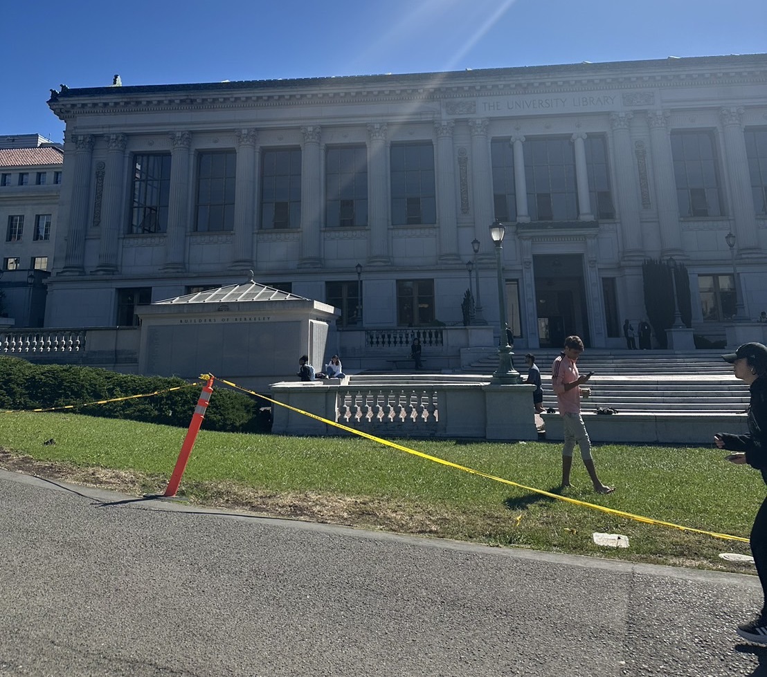
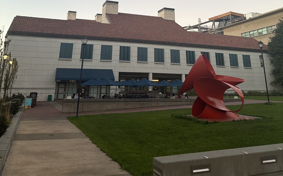
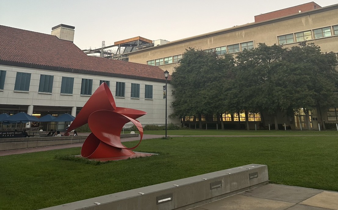
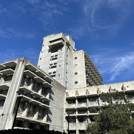
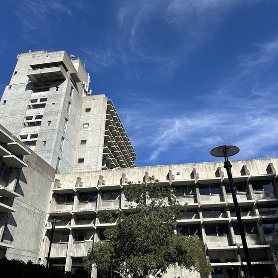
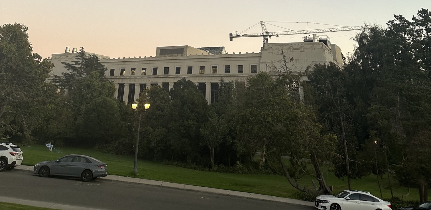
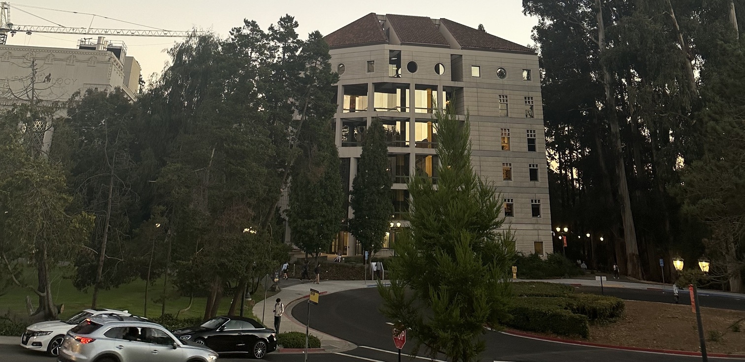
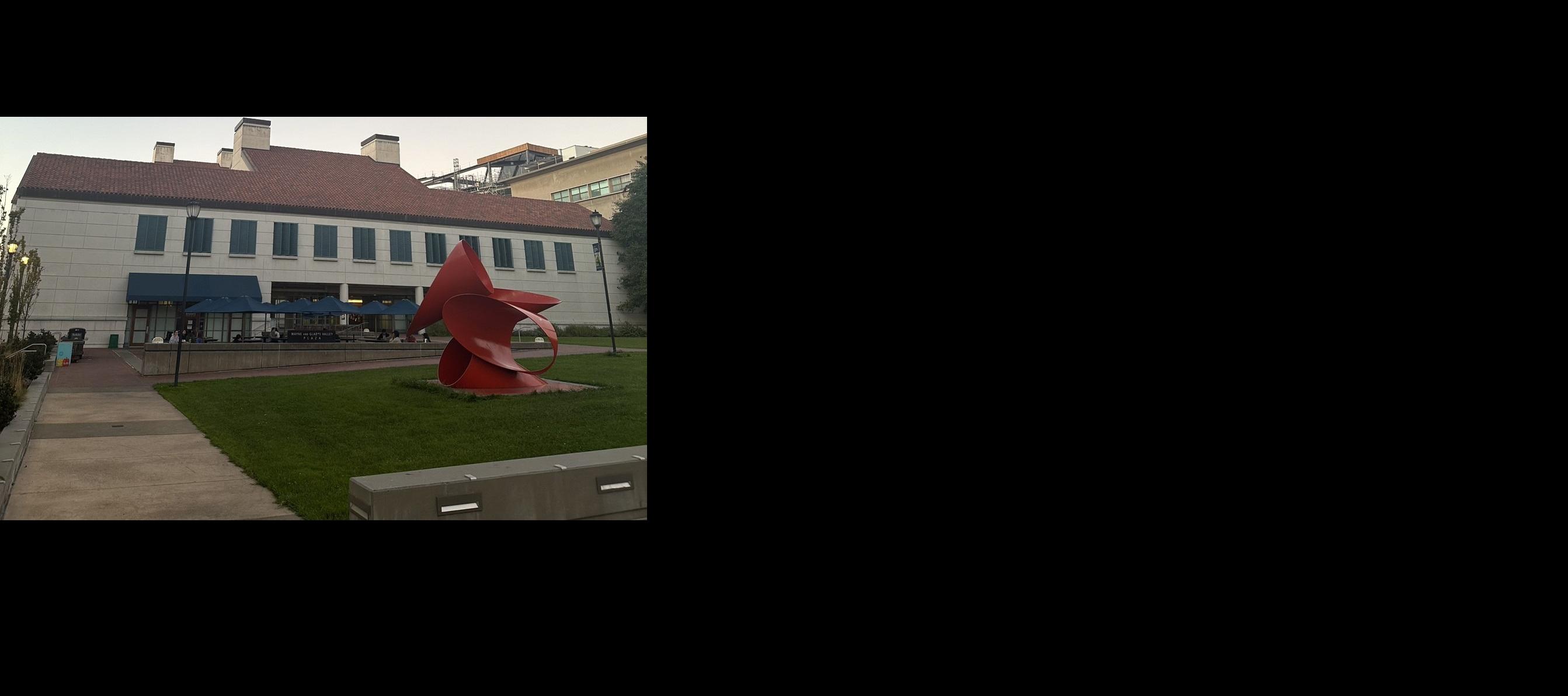
We took a few images of the scenes around Berkeley campus and the images are show below
Part 2: Recover Homographies
So the first thing we have to do is to find the correponding points between the images. This was done by using the tool from last year. Then we can use the corresponding points to find the homography matrix by using the least square method. This is done by using the equation that was set up in the class and the expandsion of the solution I look into Alec Li last year project. Specially, we need to find the homography matrix that map the source image to the target image and the equation is shown below.
\[ \begin{bmatrix} a & b & c \\ d & e & f \\ g & h & 1 \end{bmatrix} \begin{bmatrix} x \\ y \\ 1 \end{bmatrix} = \begin{bmatrix} wx' \\ wy' \\ w \end{bmatrix} \] \begin{align*} ax + by + c &= wx' \\ dx + ey + f &= wy' \\ gx + hy + 1 &= w \end{align*}
by substituing the value of w back into the equation we get the following equation.\[ \begin{align*} ax + by + c &= (gx + hy + 1)x' \\ dx + ey + f &= (gx + hy + 1)y' \\ ax + by + c - gx'x - hy'x &= x' \\ dx + ey + f - gx'y - hy'y &= y' \\ \begin{bmatrix} x & y & 1 & 0 & 0 & 0 & -x'x & -x'y \\ 0 & 0 & 0 & x & y & 1 & -y'x & -y'y \end{bmatrix} \begin{bmatrix} a \\ b \\ c \\ d \\ e \\ f \\ g \\ h \end{bmatrix} &= \begin{bmatrix} x' \\ y' \end{bmatrix} \end{align*} \]
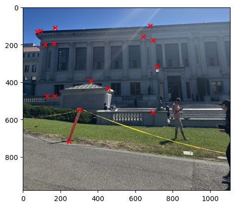
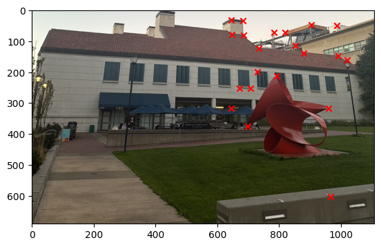
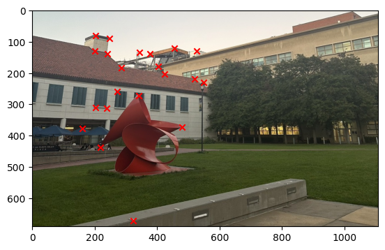
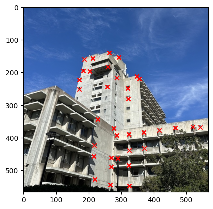
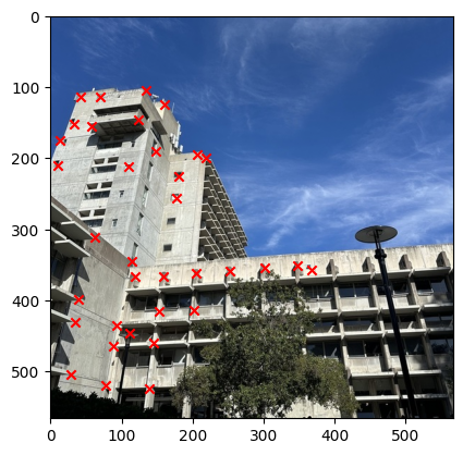
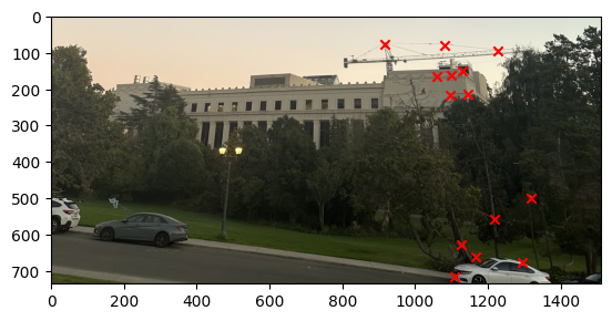
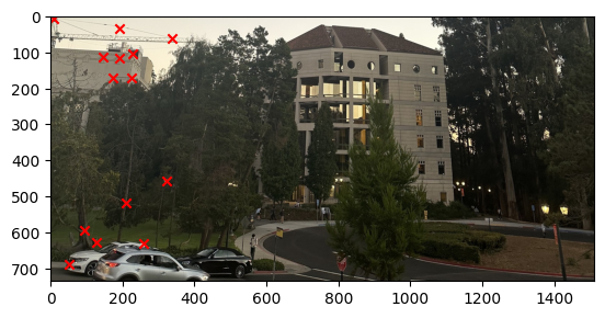
We can then stack all the points together and then use the least square method to solve for the homography matrix and get the solution. The image below show the result of correponding points for each image.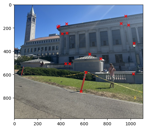
Part 3: Image Warping
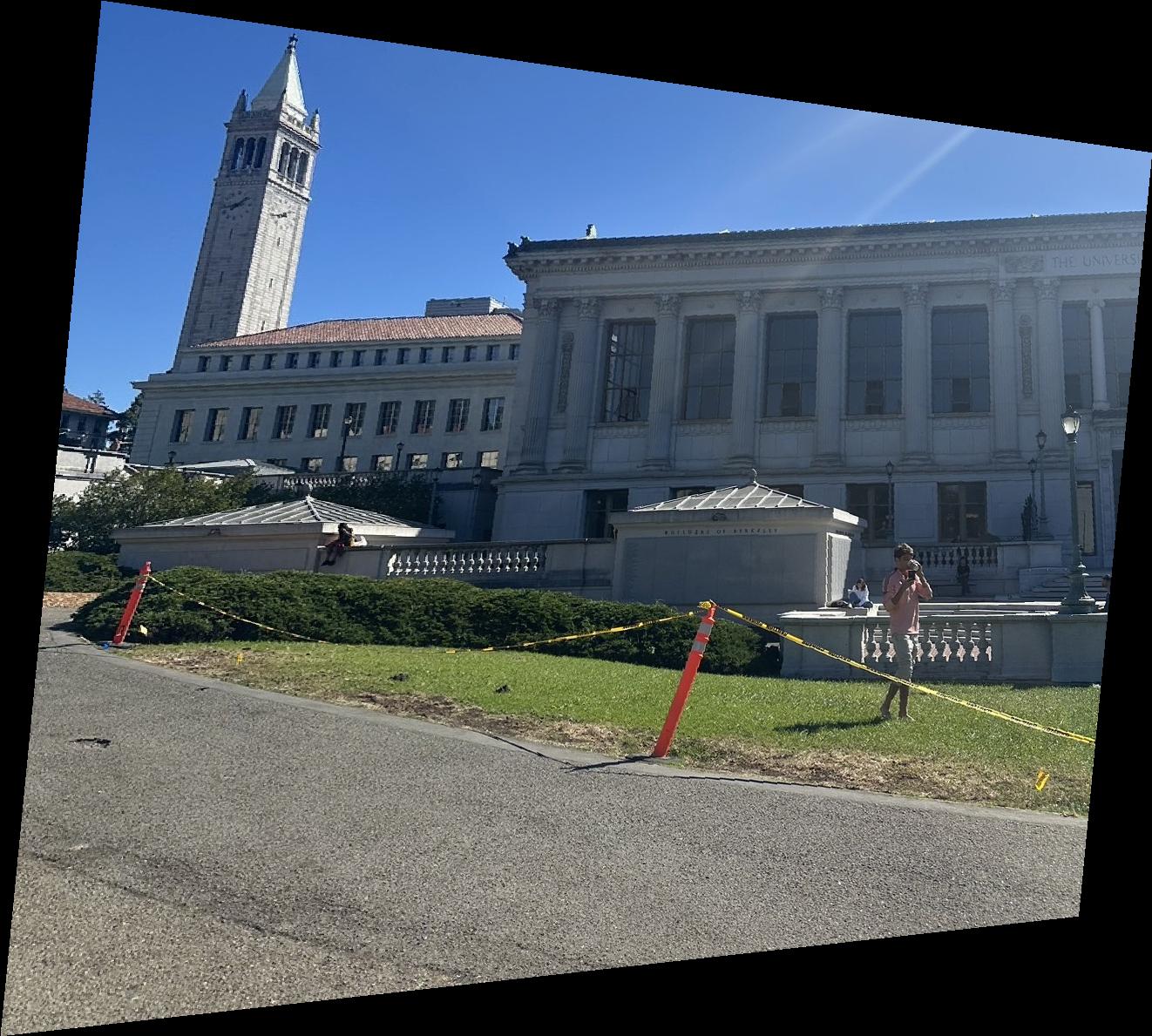
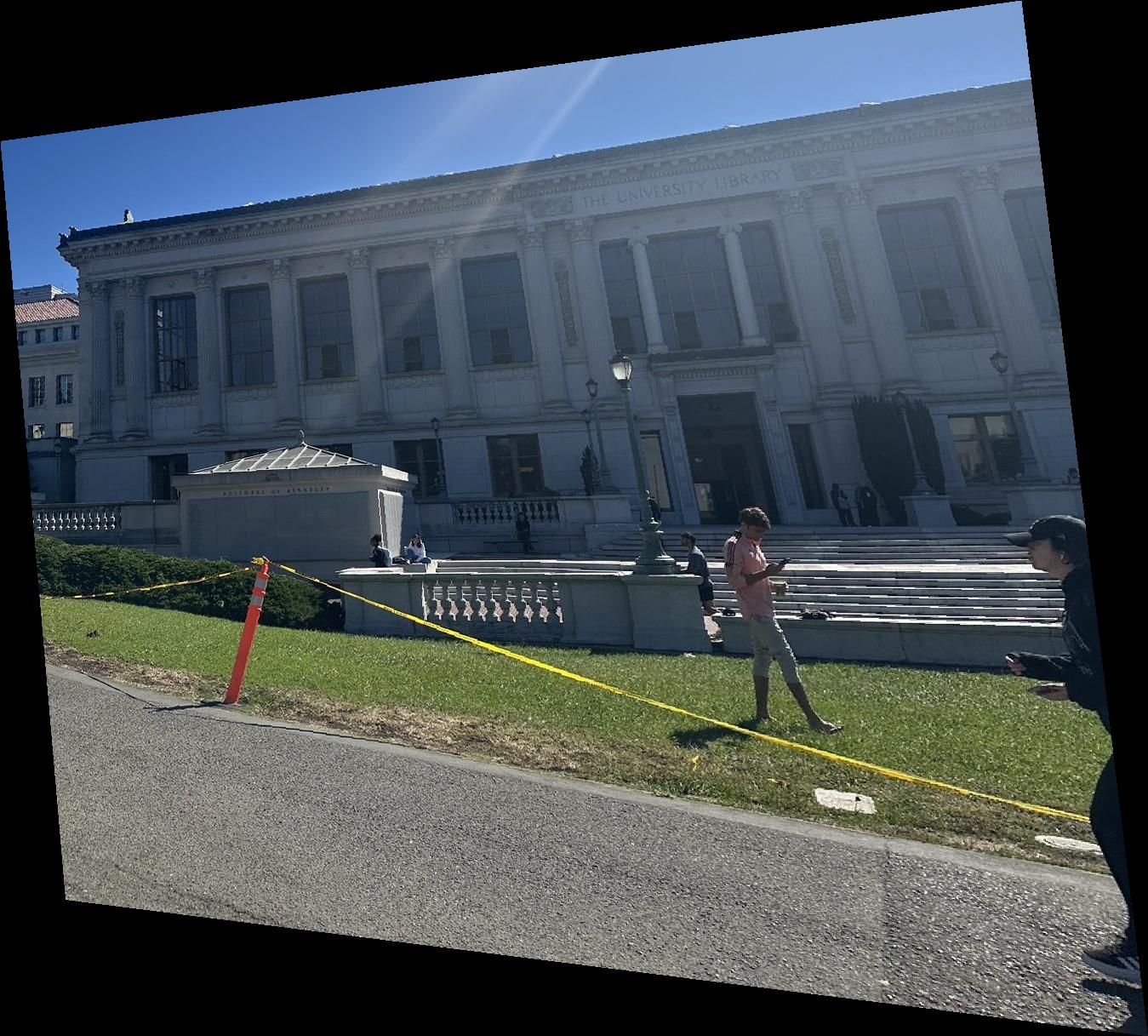
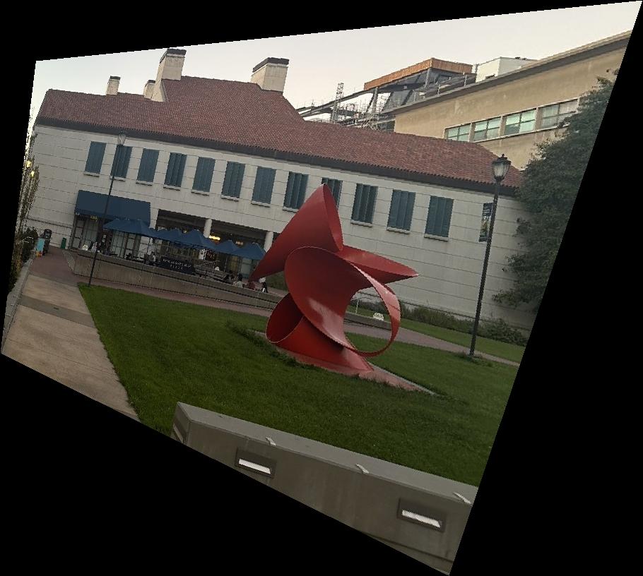
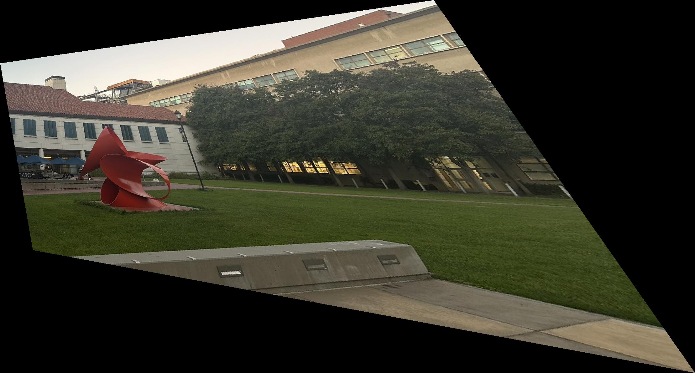
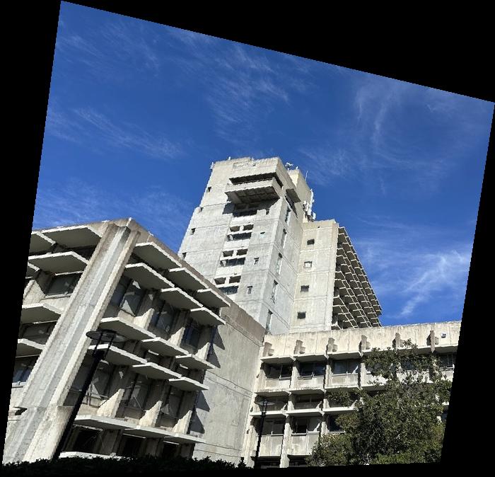
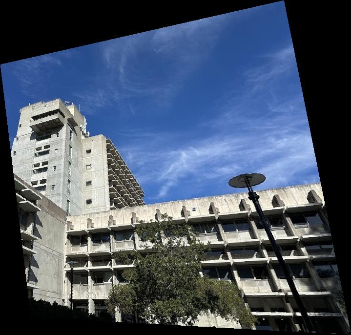
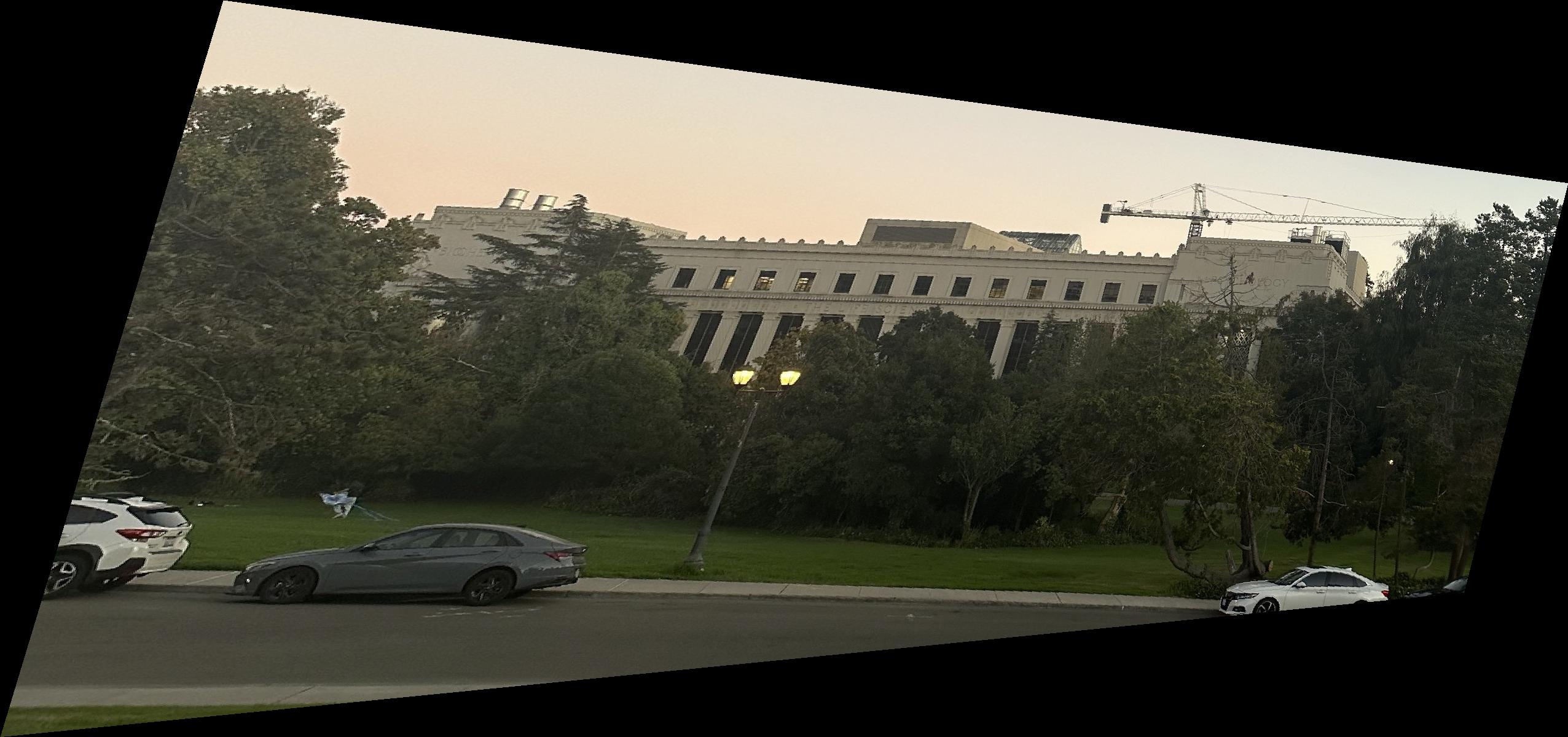
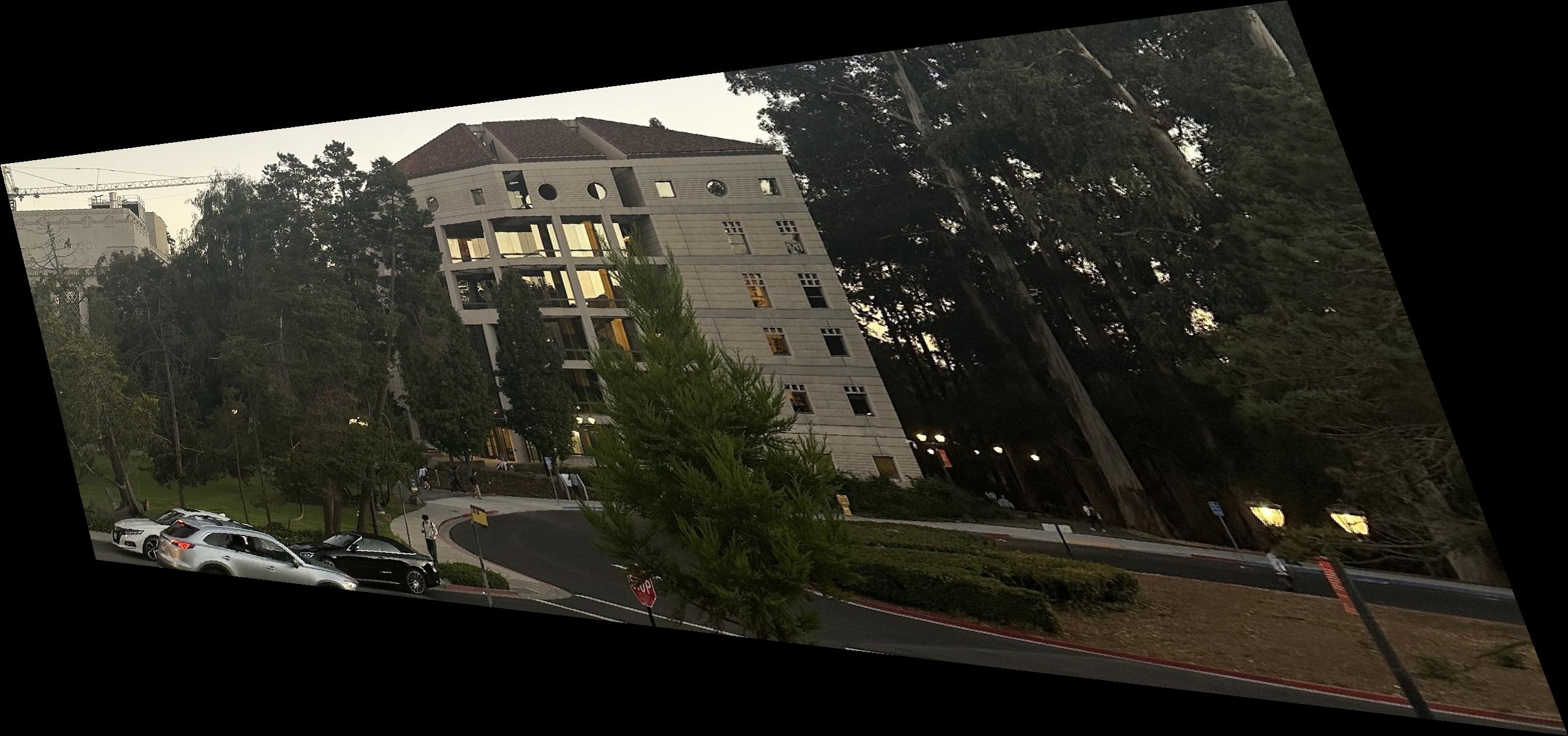
Now that we have the homography matrix, we can use it to warp the image and this is done by firstly we have to map the corners of the source image to the target image so that we can find the size of the warped image. Then we have to get the new canvas where this is calculated from the target corners. Then we use something that is very similar to the previous project where we do the inverse warping and then use the grid data to get the pixel value and return the pixel value to the new canvas. The image belows show the result of the warped image where I warp the first image to the second and I also showed the second image warped to the first image as well.
Part 4: Image Rectification
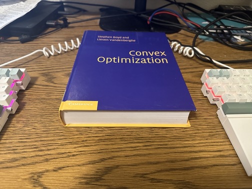
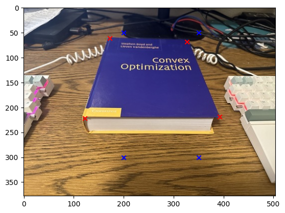
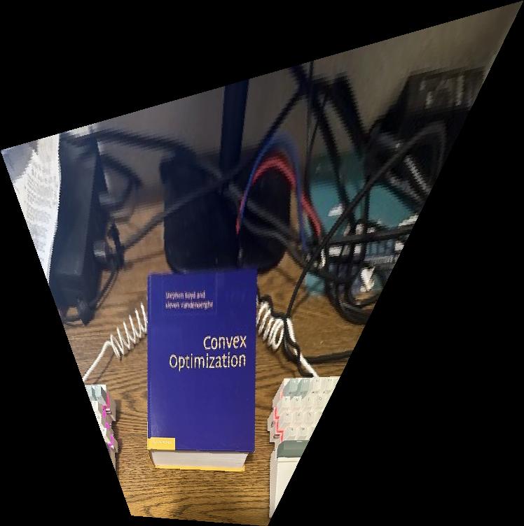
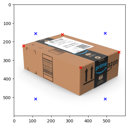
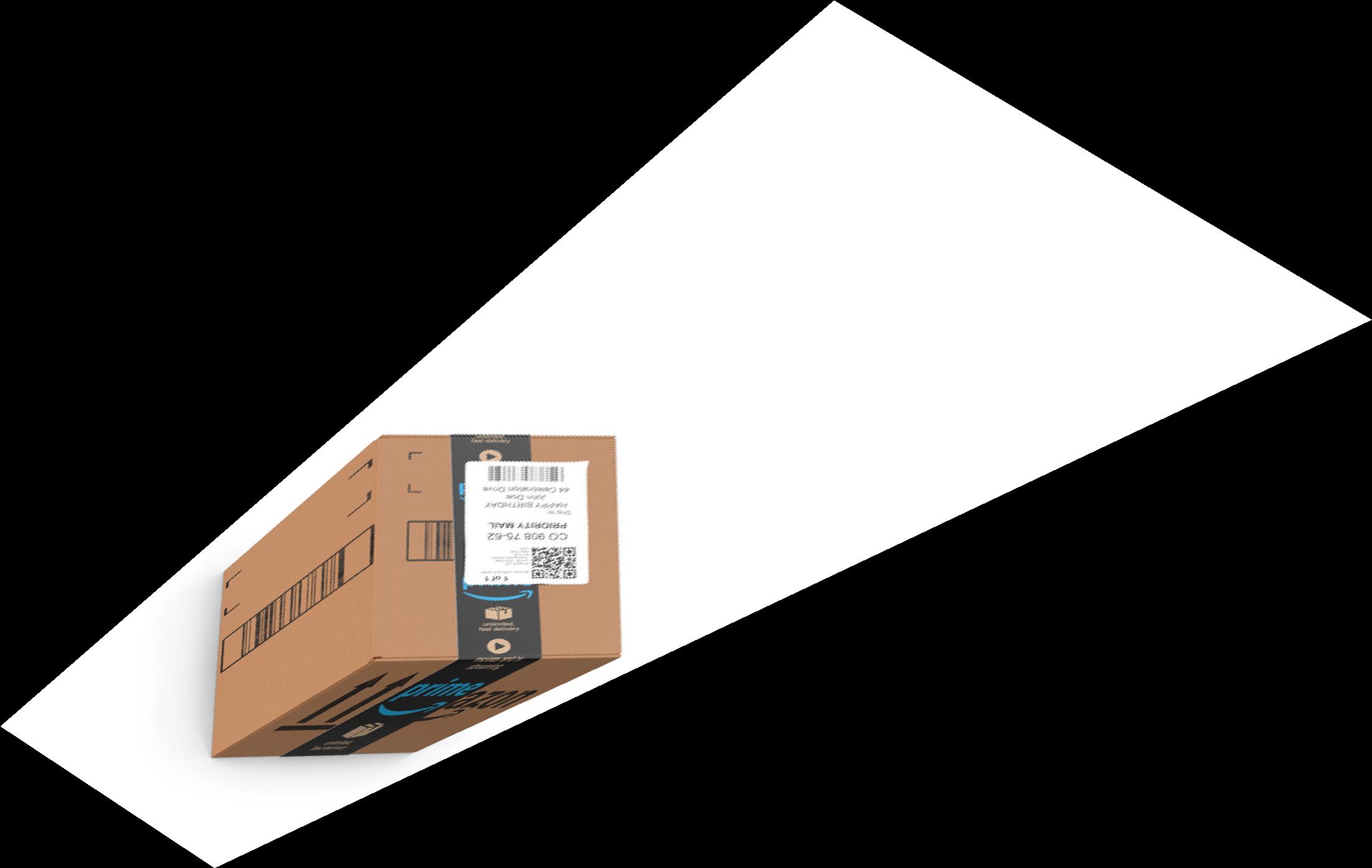
Now that we have the homography matrix, we can use it to rectify the image. However, as we can see that there is only one image therefore I decided to define the corresponding points to the same image itself. The image below show the immediate result where the red points are representing the source point and the blue point represent where we want to map the source point to. Addtionally we also show the result of the rectified image. We note here that the first image is the photo I took by myself and the second image I got it from this website amazon package

Part 5: Blend the images into a mosaic
Now that we have the homography matrix, we can use it to rectify the image. The first thing we have to do is that since the image that is being warped is not the same size as the sorce image, which therefore mean that we have to pad the image so that it is the same size and also we want to make sure that the image is also align with each other as well. Note that in our case we use the left image as the base and the right image to warp to the left image. The image below show the result of the padded image for each image and as we can see that the image is align and also same size.
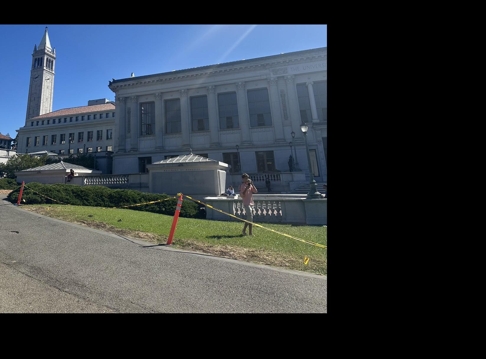
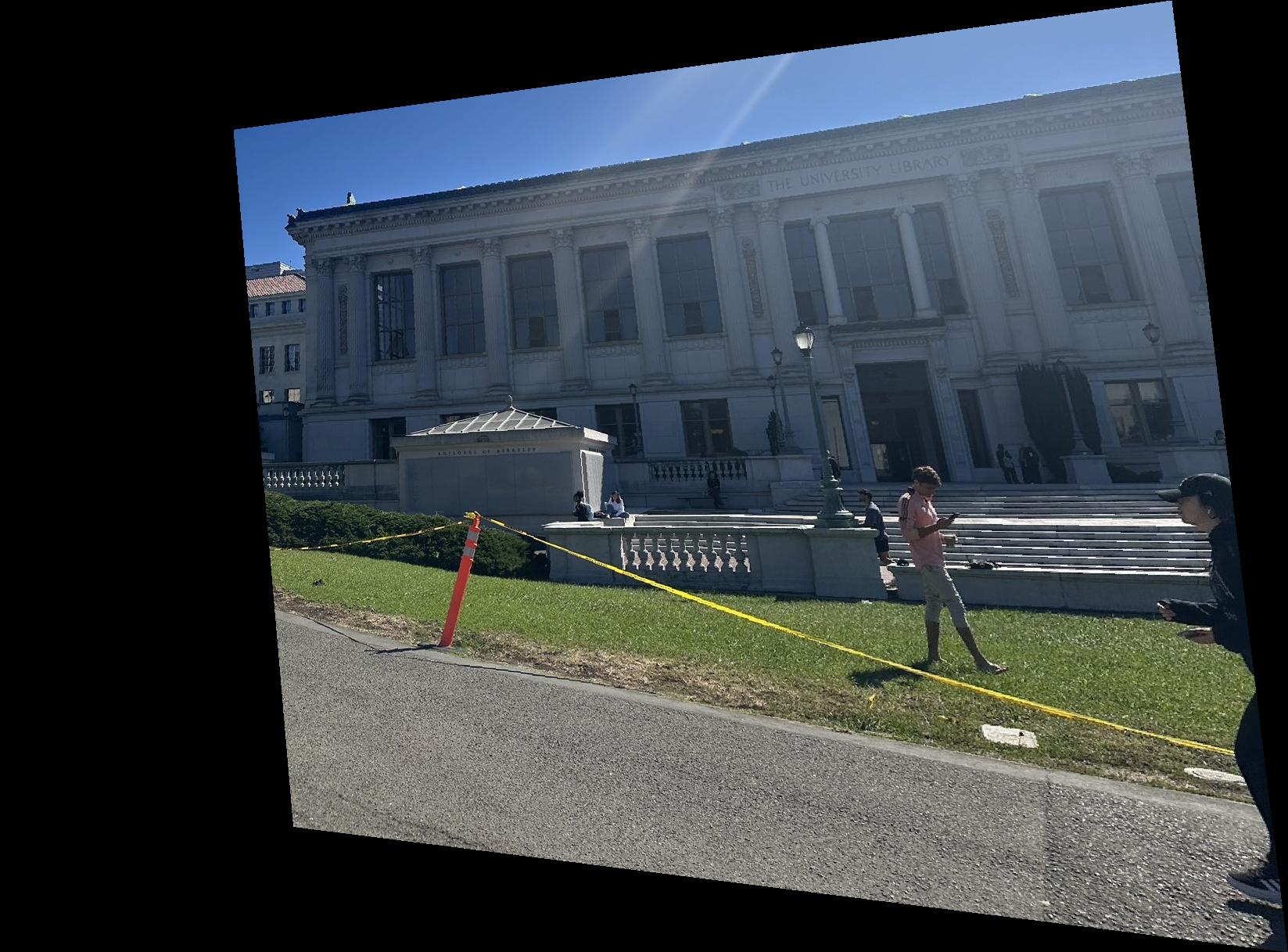
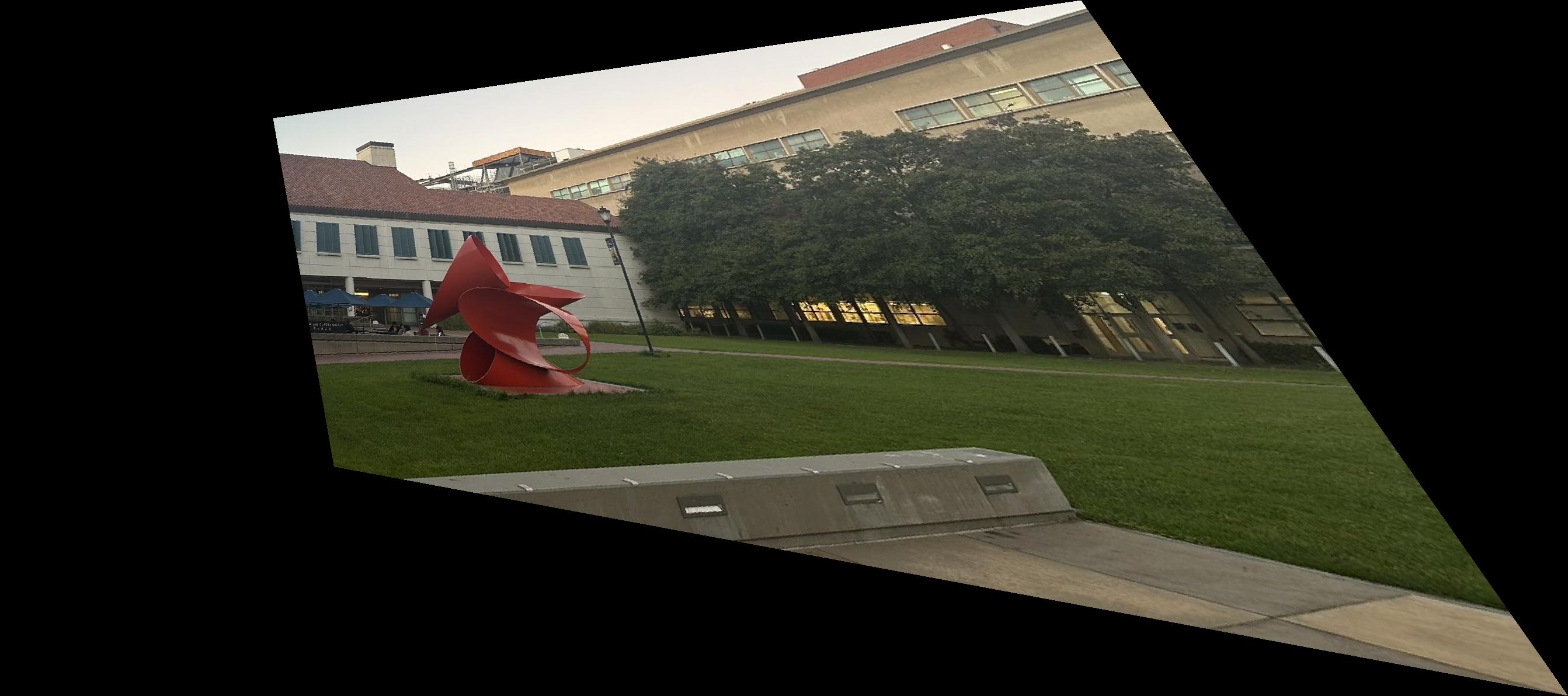
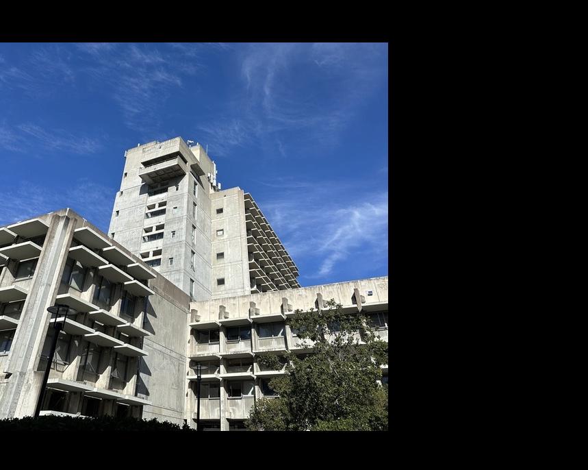
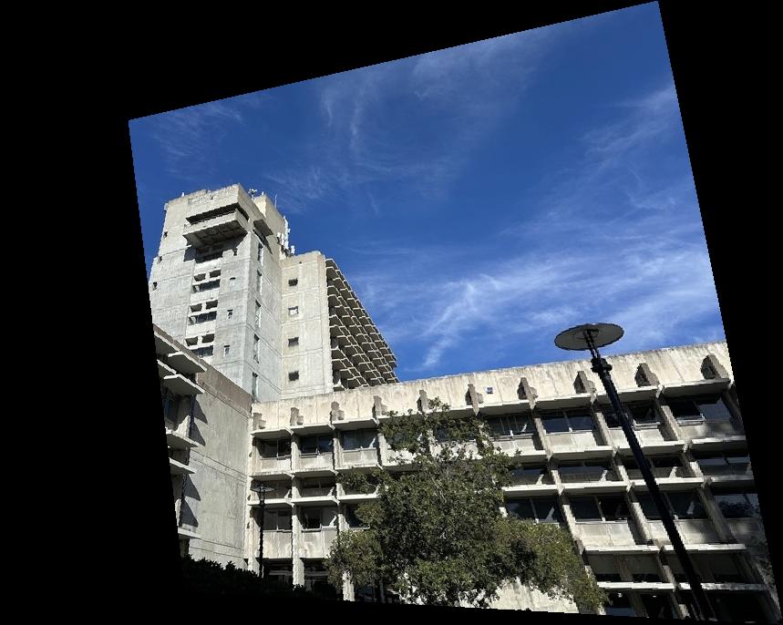
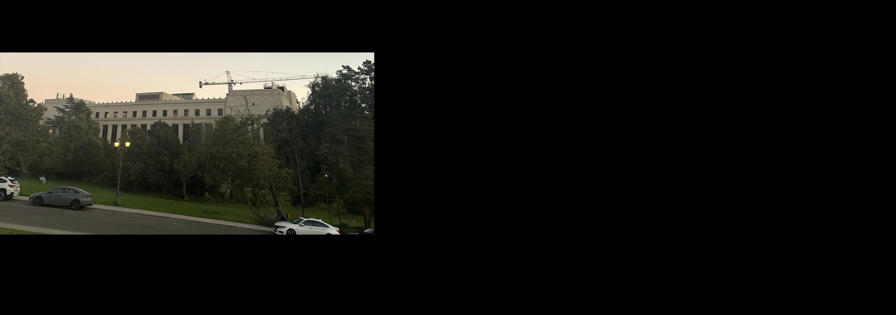
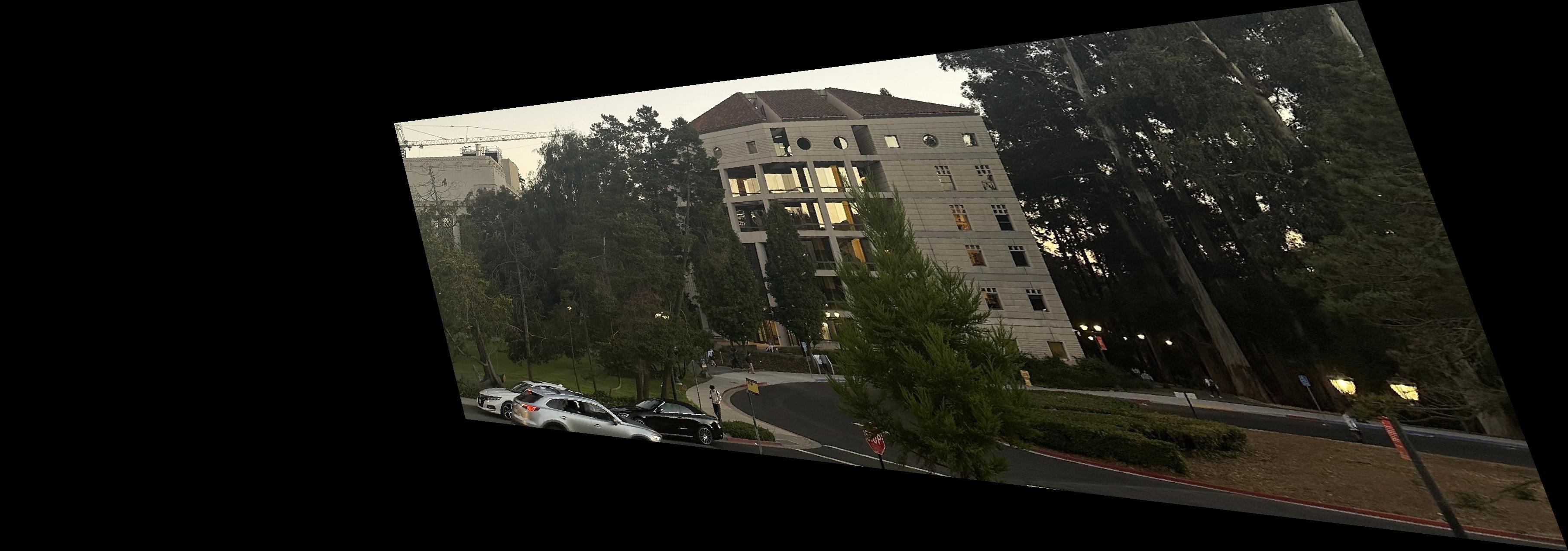
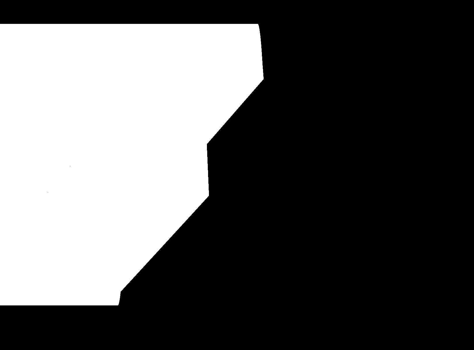
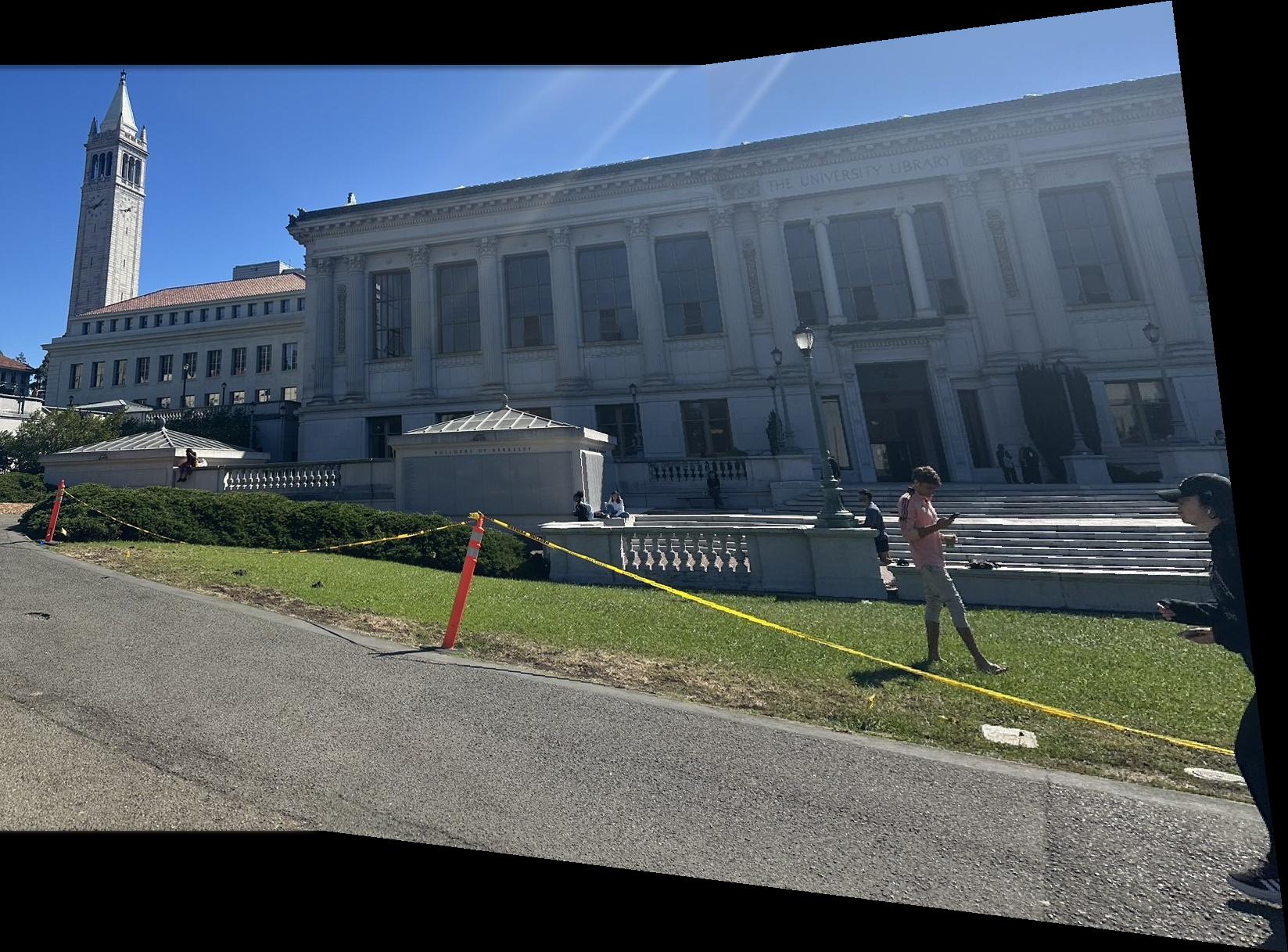
We then tried to use the mask in the lecture that is wherever there is only pixel from first image we set that to be 1 and whenever there are intersection between the two images then we set the mask to be 0. Then after that we do the interpolation of this mask with the base image and the warped image. The image below shows the result of both the mask and the mosaic image.
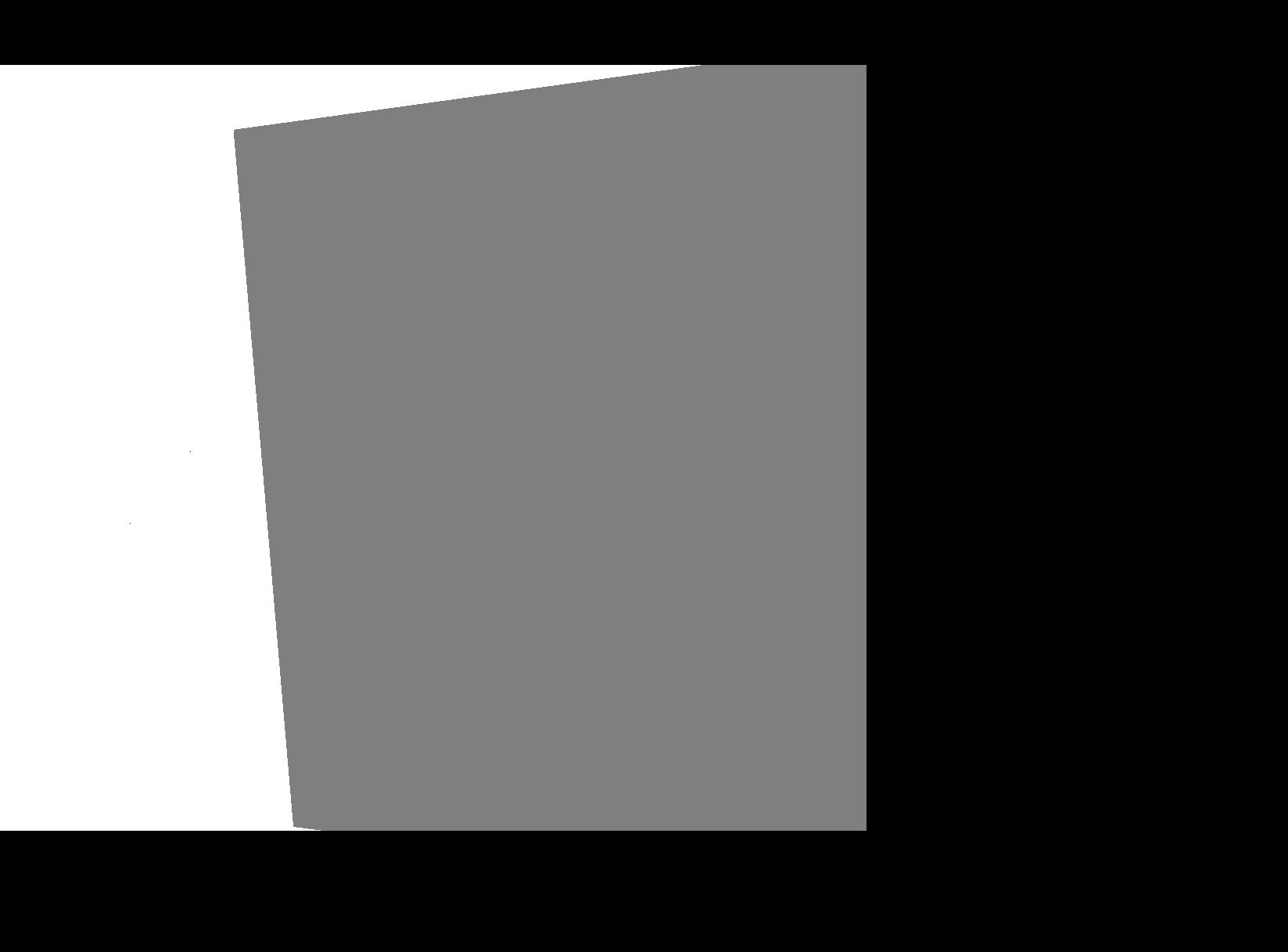

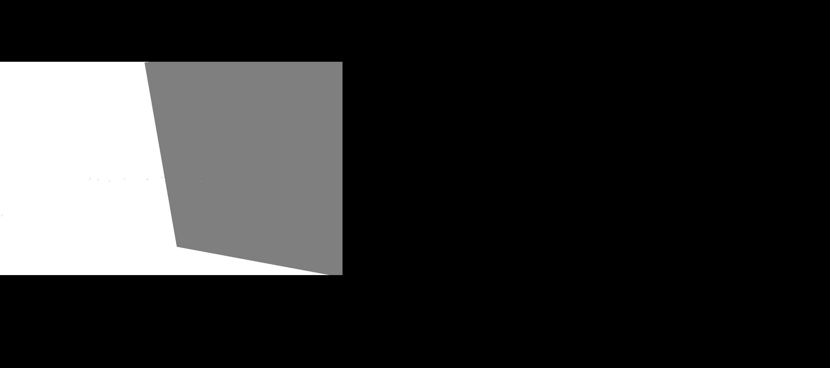
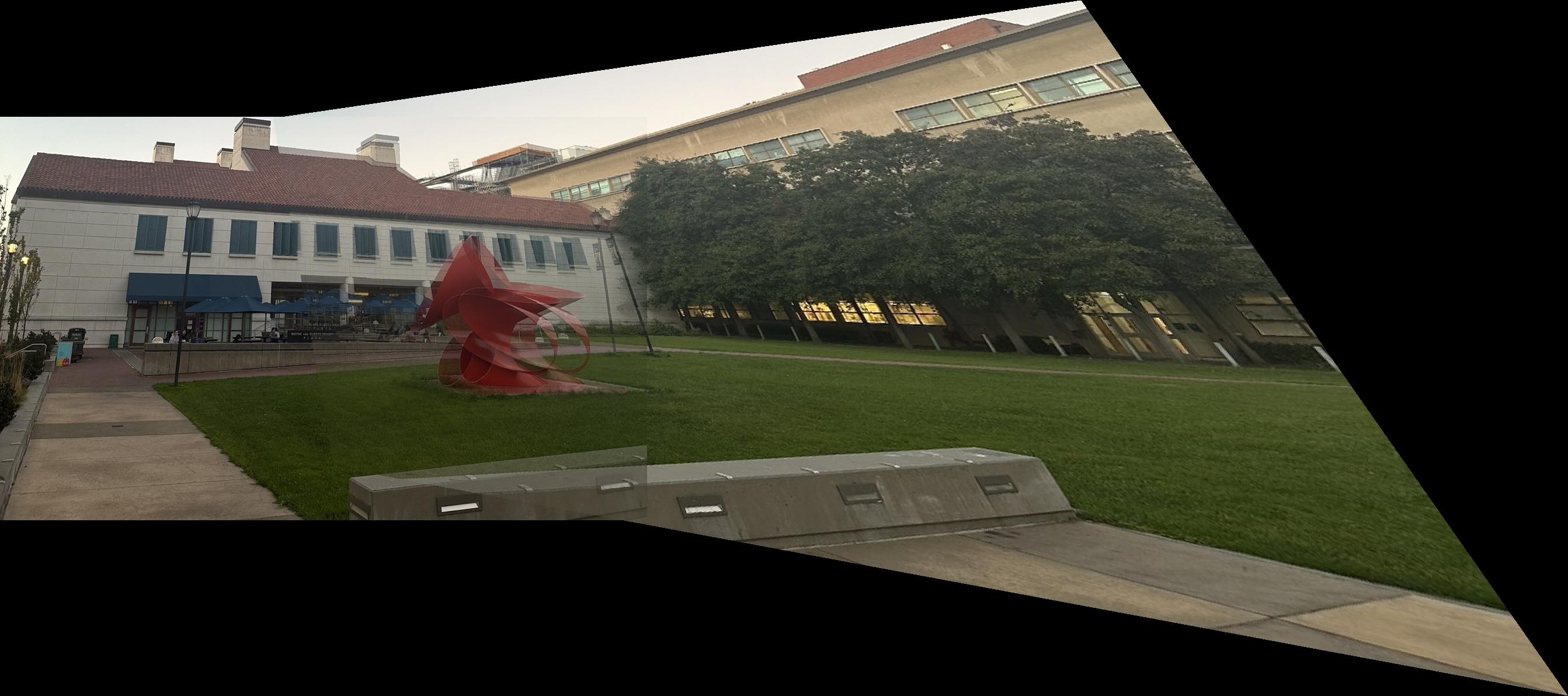
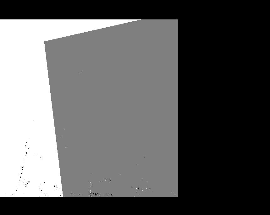

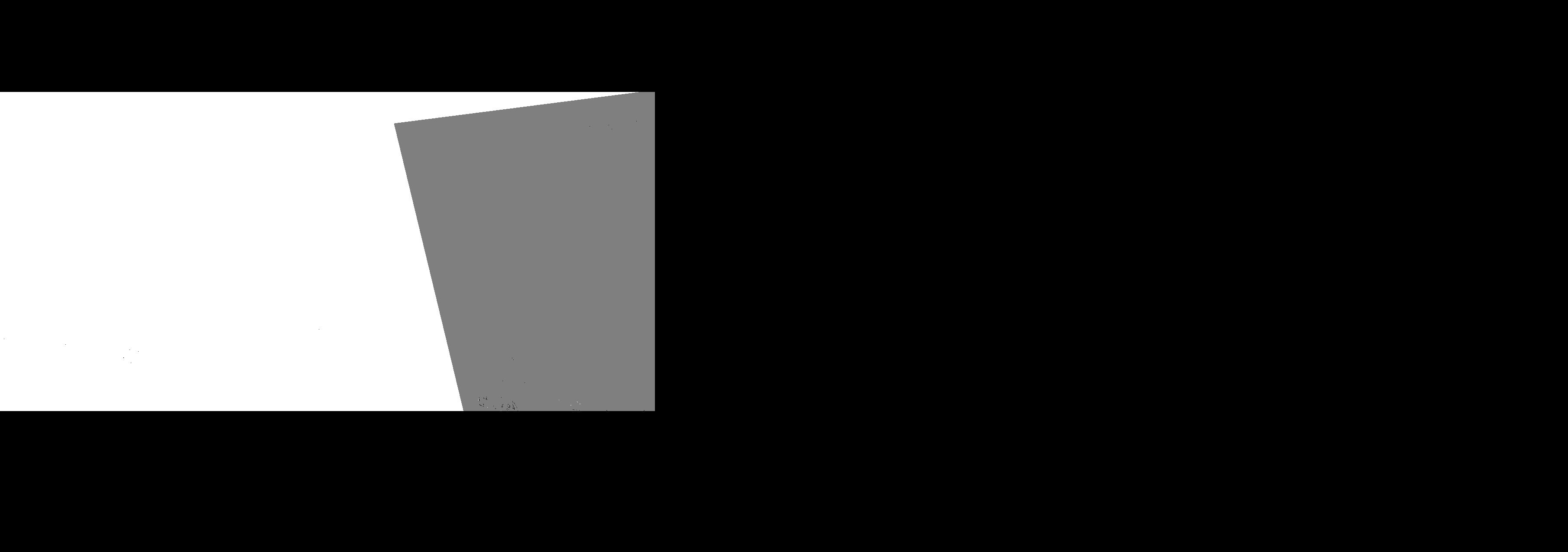

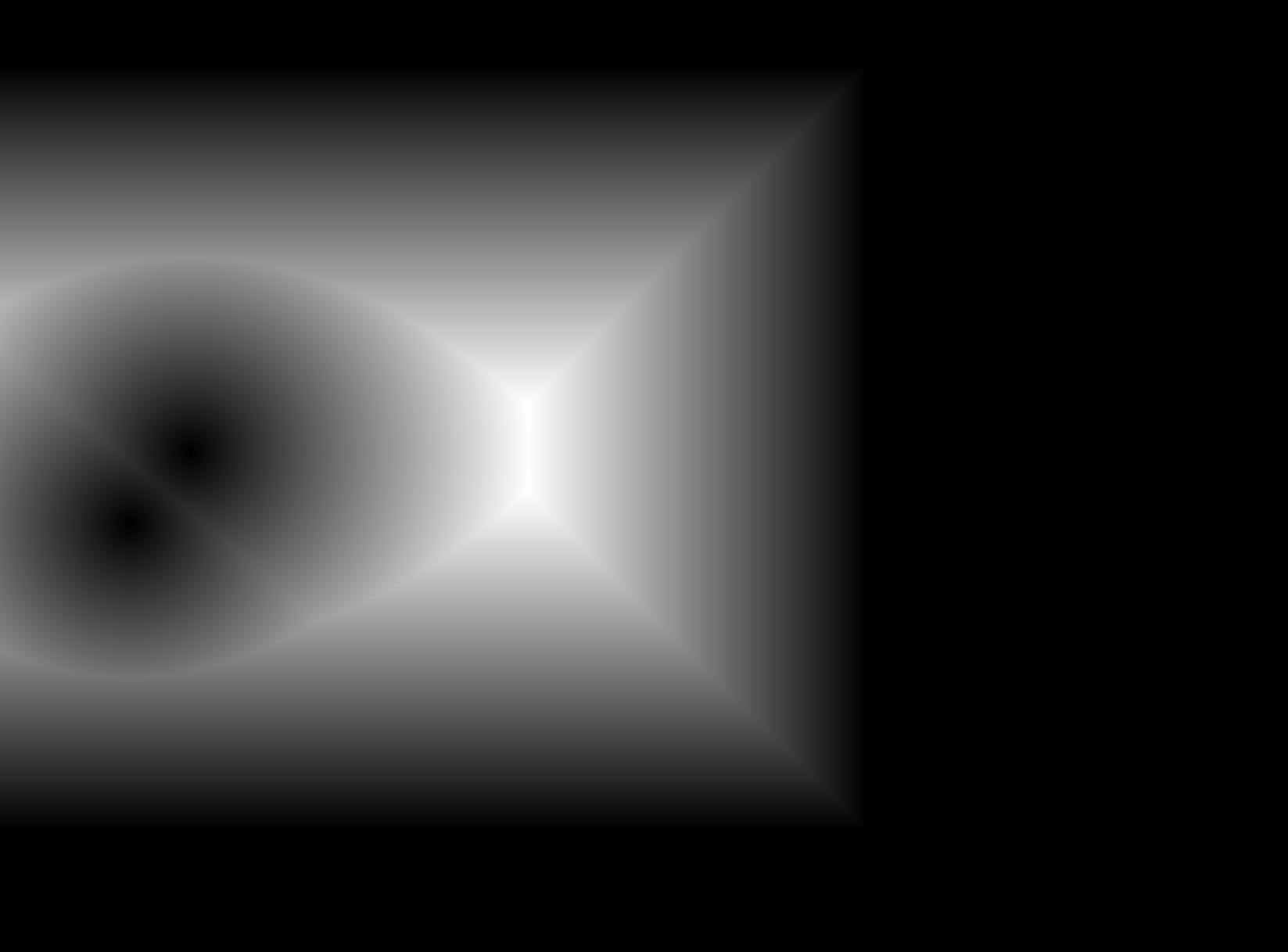
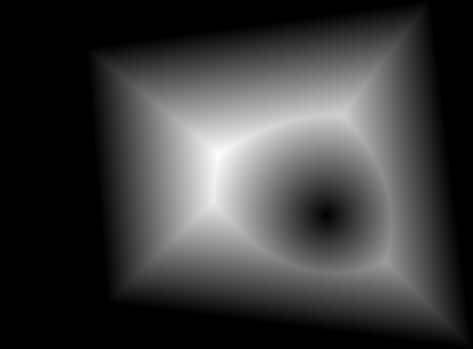
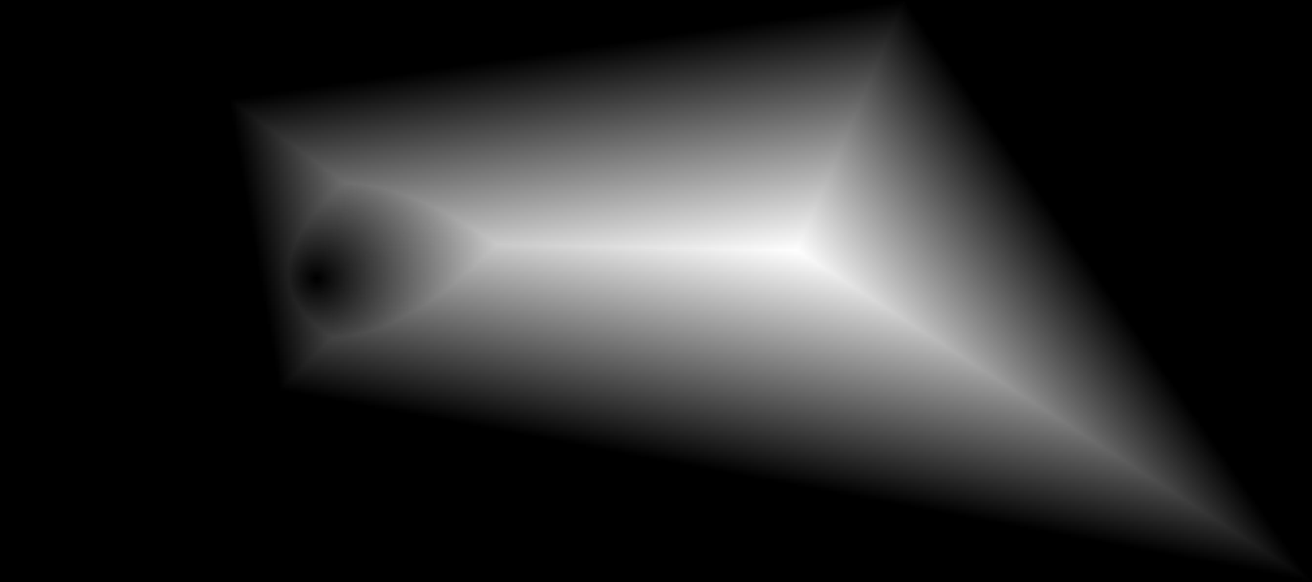
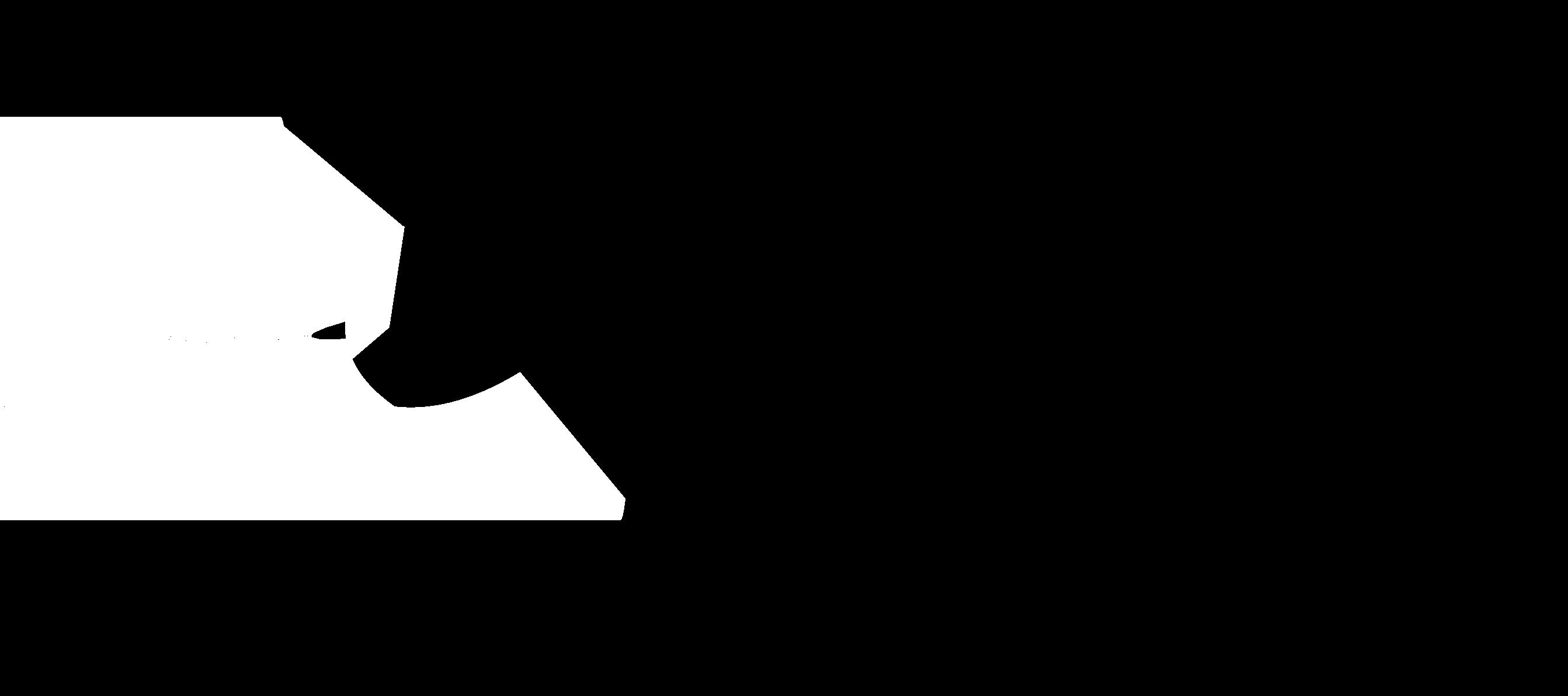
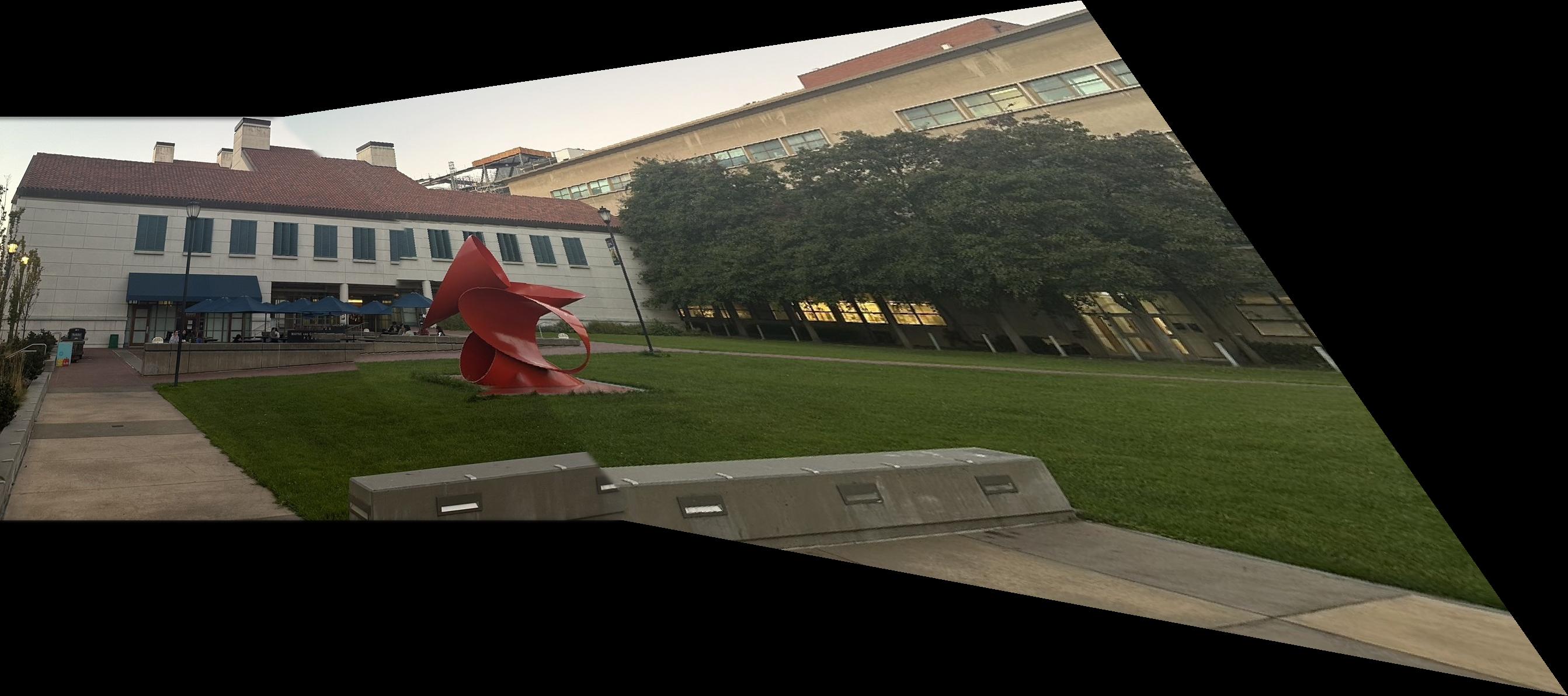
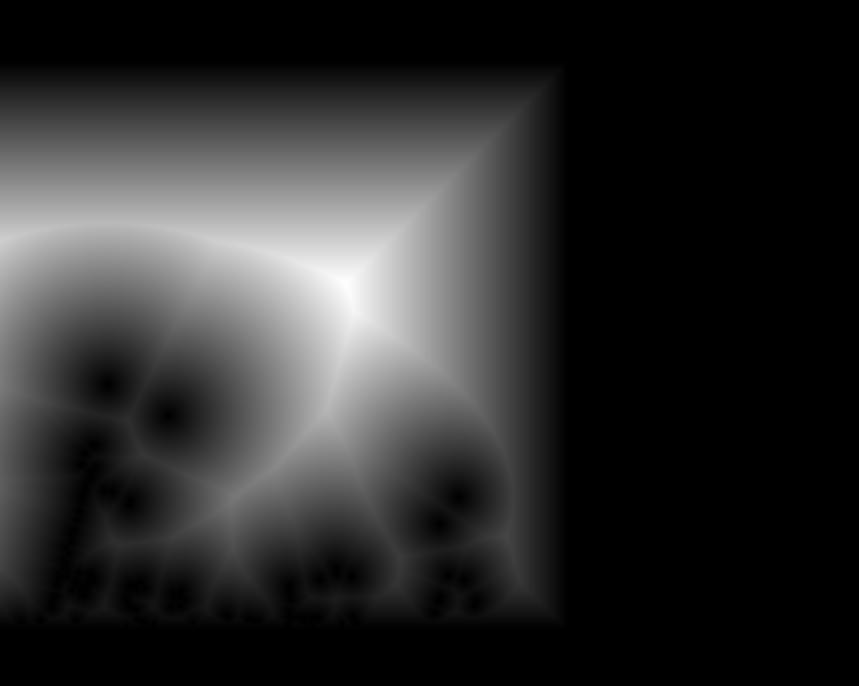
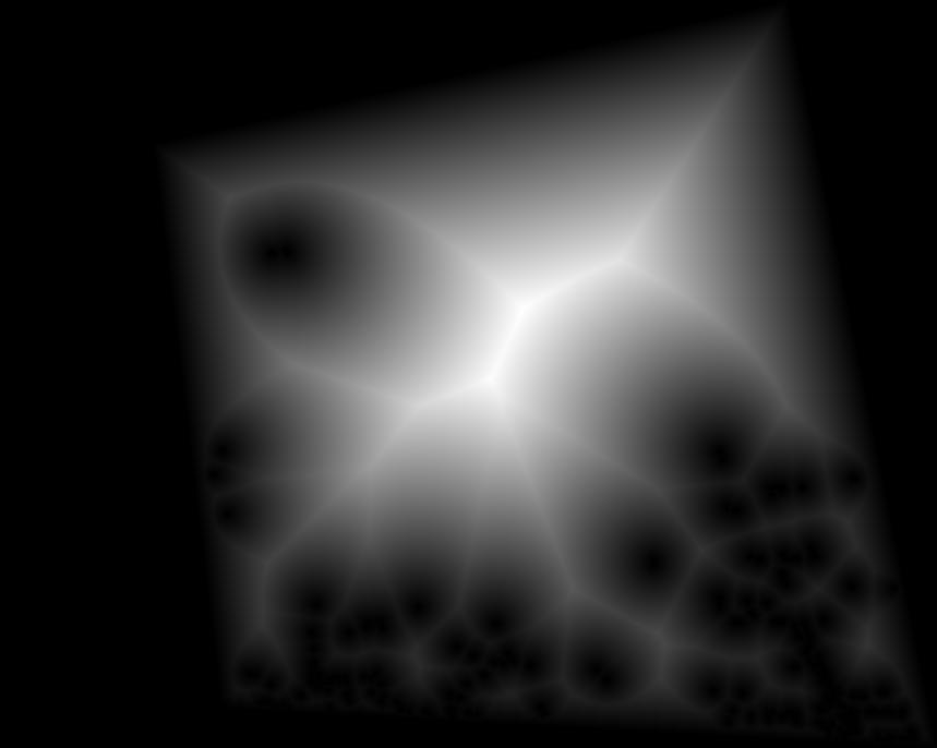
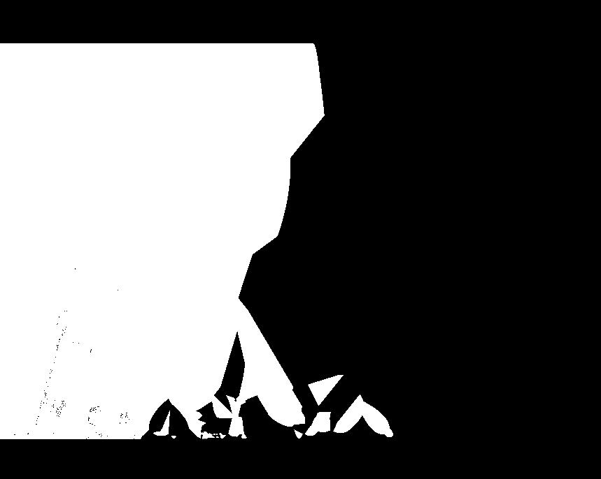
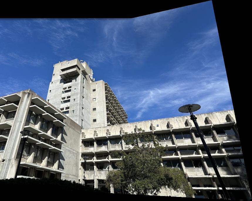
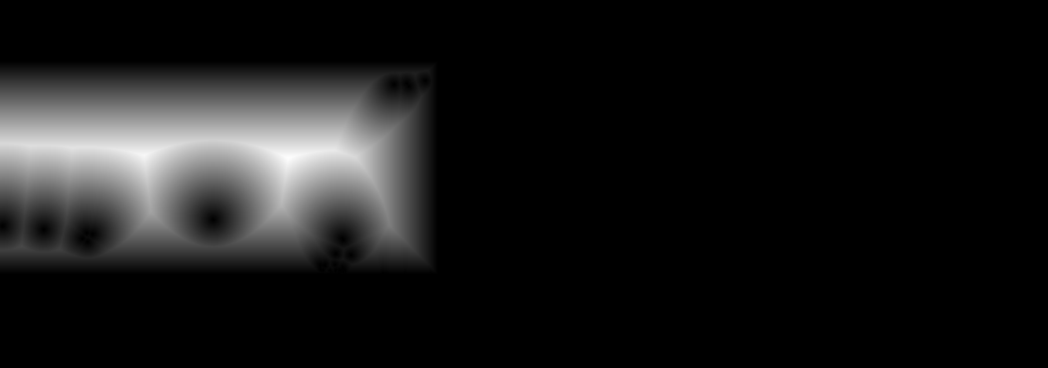
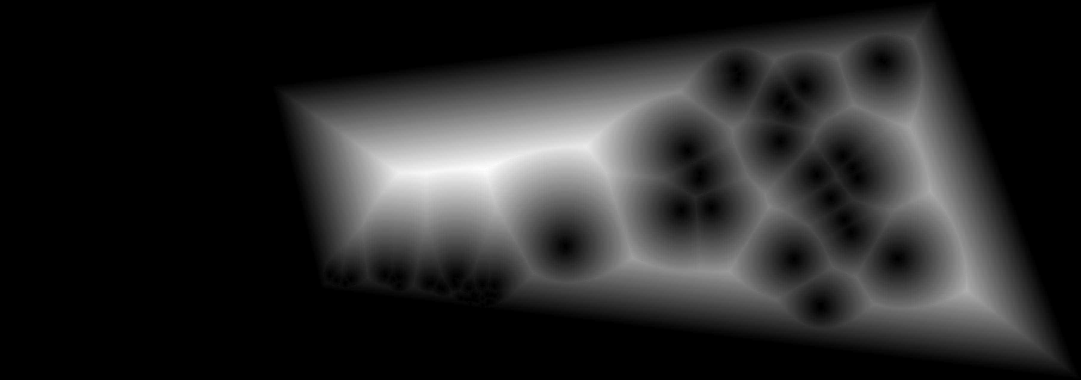
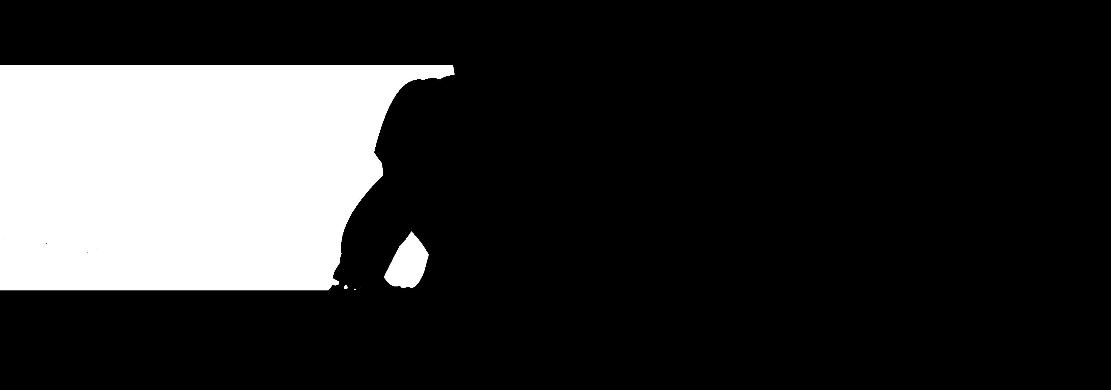
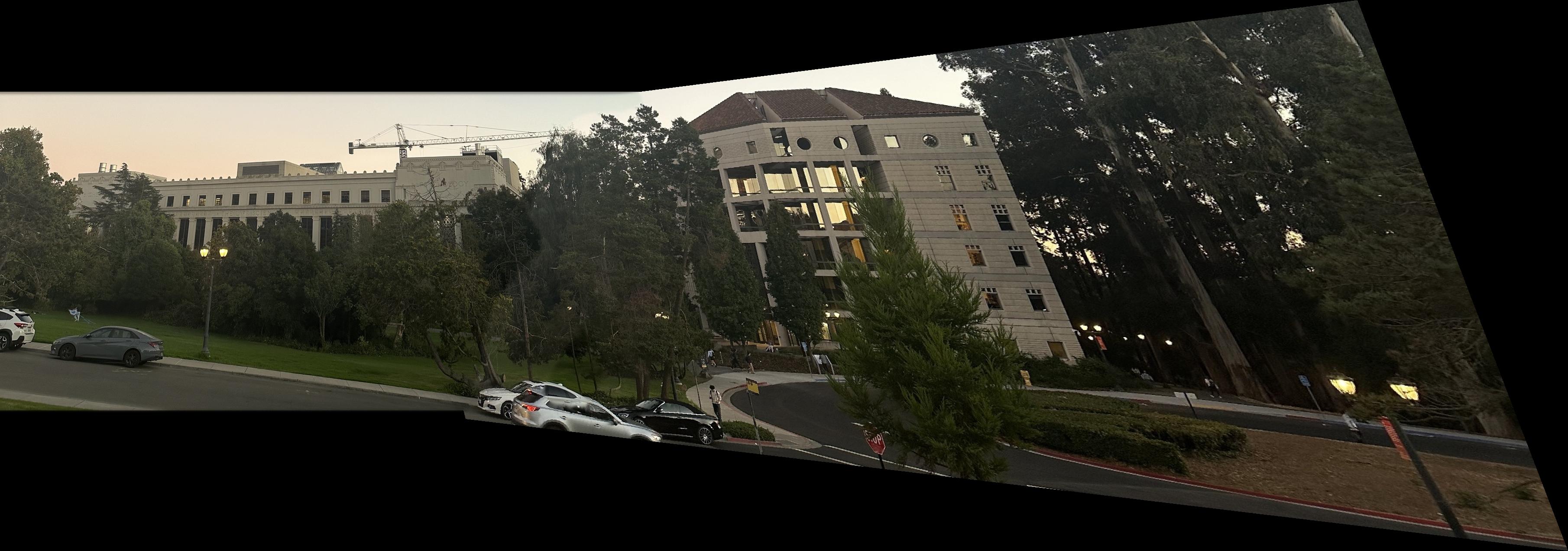
However, as we can see that the image is not as clear as it should be and also there seems to be some artifacts in the image. Therefore, we will try to fix this by using the bwdist function that was given in the lecture where we create the two mask base on the bwdist and then the last mask is the one such that the pixel value is closer to the first image. Then after that we used the gaussian pyramid to blend the image together and we show the final mask and also the final mosaic image.

Project 4B
For this part we will do feature matching for autostitching. We will start first with Harris Intterest Point Detector then we implement the Adaptive Non-Maximal Suppression and then we implement feature descriptor extraction then we implement the feature matching and at the end we use the RANSAC for more robust matching and then we make the image mosaic.
Part 1: Harris Interest Point Detector
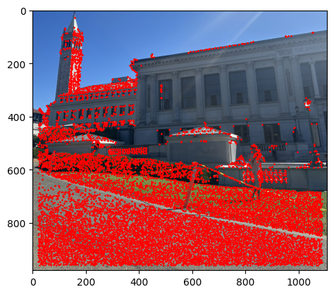
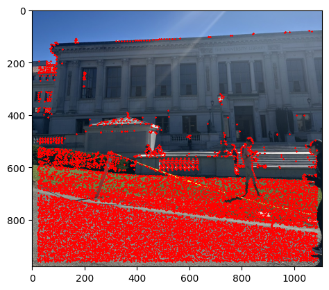
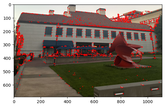
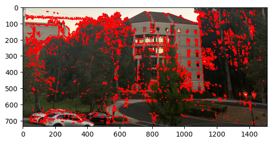
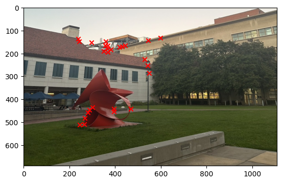
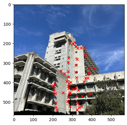
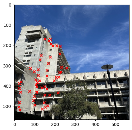
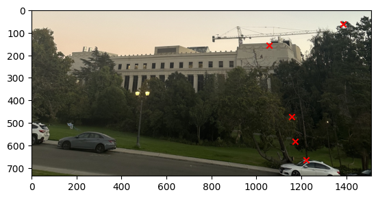
I started to get the Harris Interest Point Detector by first using the code that was given. Where we set the edge discard to be more than 20. Then running the result on the image we get that there were too many points that were detected. Therefore, I decide to set a threshold for the corner response to be 0.1 and then we get that there are only about 11,000 points. The image below shows the result of the Harris Interest Point Detector.
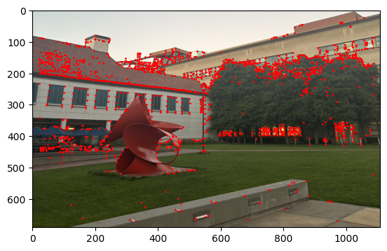
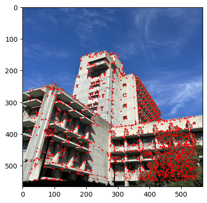
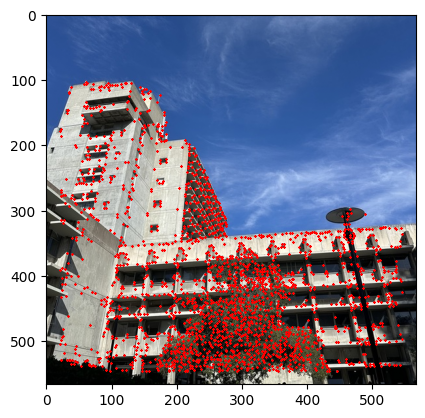
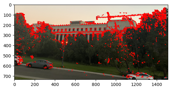
Part 2: Adaptive Non-Maximal Suppression
Now that we have the Harris Interest Point, we can see that there are still too many points that are detected. Therefore, we will still have to do the Adaptive Non-Maximal Suppression to filter the number of key points that we have. Essentially, the algorithm will assign every key point an r score where the function f is the corresponds to the corrner response. We have the following equation.
Here is the equation:
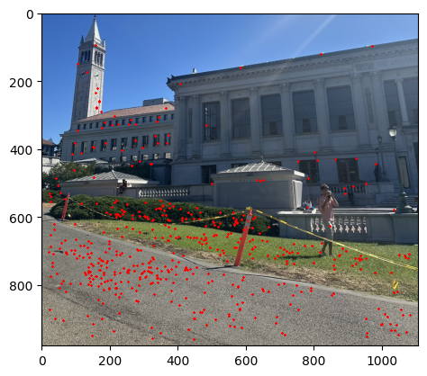
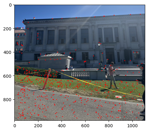
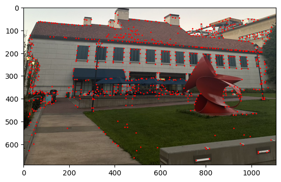
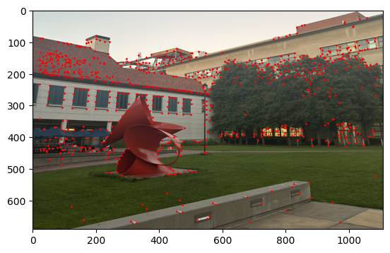
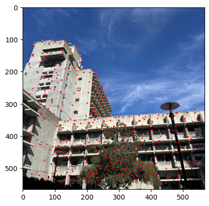
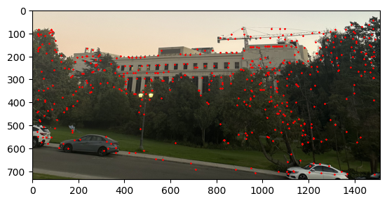
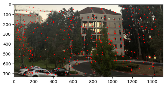
Then we pick the 500 points that has the highest r scores as the output. The image below shows the result of the Adaptive Non-Maximal Suppression.

Part 3: Feature Descriptor Extraction
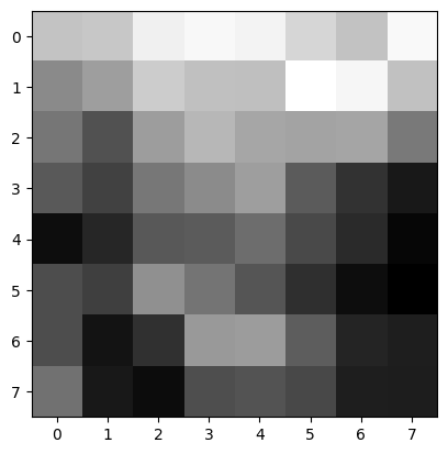
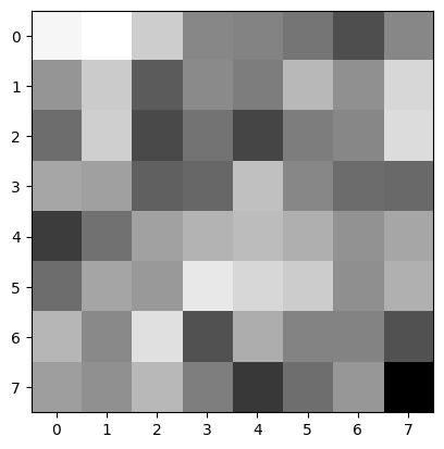
Now after we have the 500 points from the Adaptive Non-Maximal Suppression, we still need something more than just a single pixel of information. Therefore, we will look into extracting the local information about the image around the key points. We captured 40x40 patch center around each key point and then we downsampled this image to 8x8 patch and we also did the normalization of the image. The image below shows the result of the Feature Descriptor Extraction.
Part 4: Feature Matching
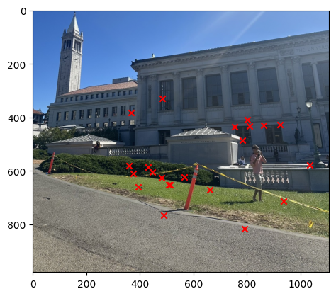
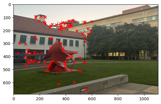
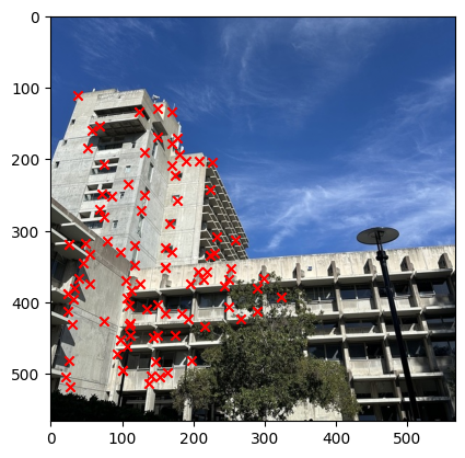
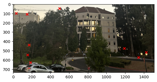
Once we get the image descriptor, then we have to use this to get the matched key points between the pairs of images. In order for us to do this, we have to use the L2 distance to find the closest key points between the two images using the Lowe's ratio. The Lowe's ratio is defined as the ratio of the distance between the closest key point and the second closest key point. If the ratio is less than 0.4 then we consider this to be a match. The image below shows the result of the Feature Matching.




Part 5: RANSAC
Now that we have the matched key points, we still do have that the there are still some outlier therefore we have to use the RANSAC to get the more robust matching. Using the following steps
- We select 4 random points from the matched key points
- We then calculate the homography matrix using the 4 points
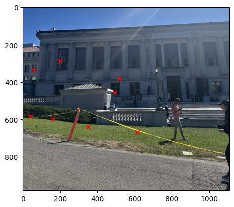
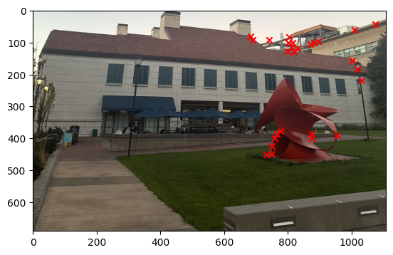
- We then use the homography matrix to warp the points from the first image to the second image and we find the inliers point pairs such that the distance between the warped points and the second image is less than 1 pixel.
- We then repeat the above steps for 2000 times and then we select the homography matrix that has the most inliers.


Part 6: Image Mosaic
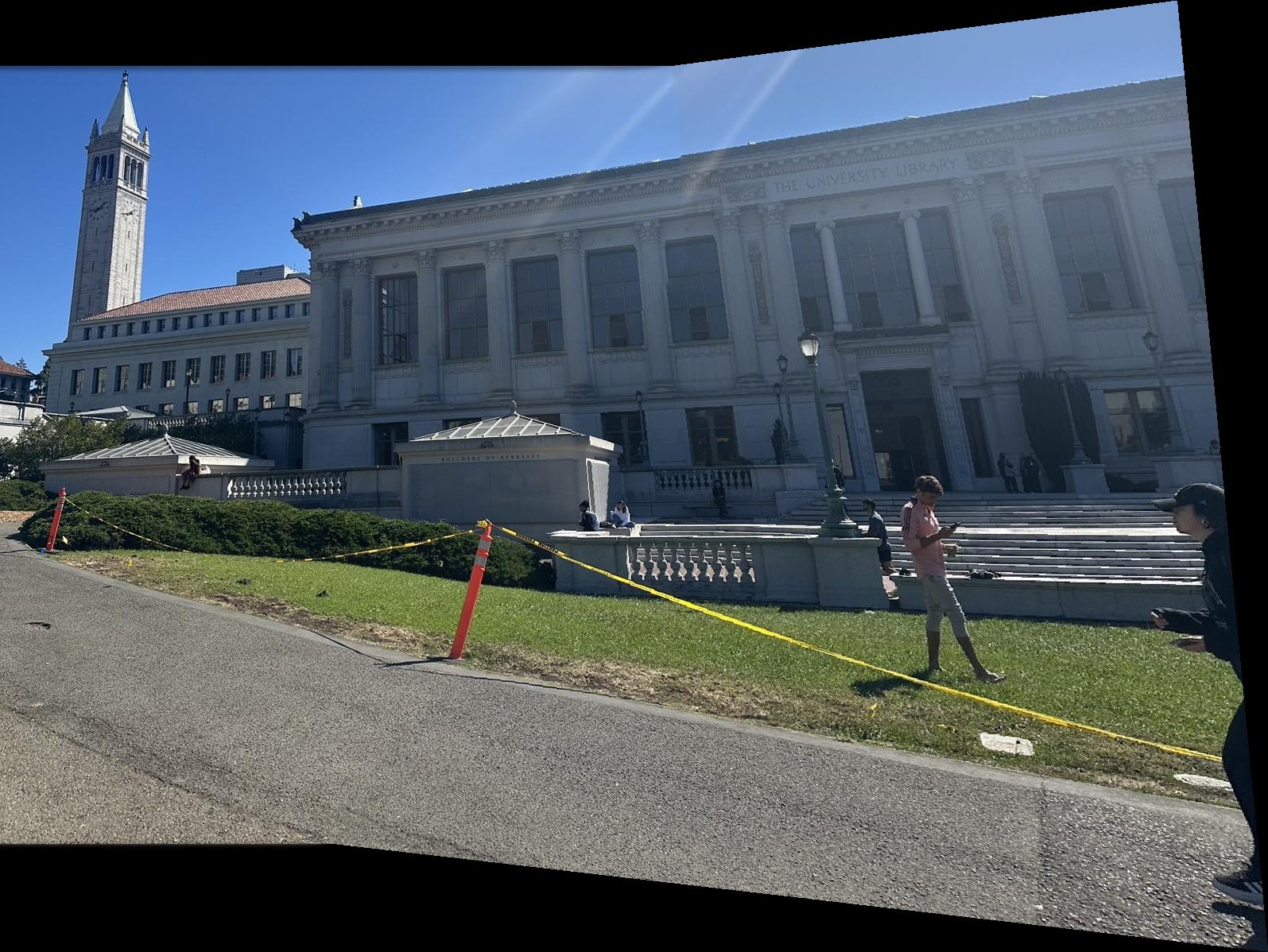
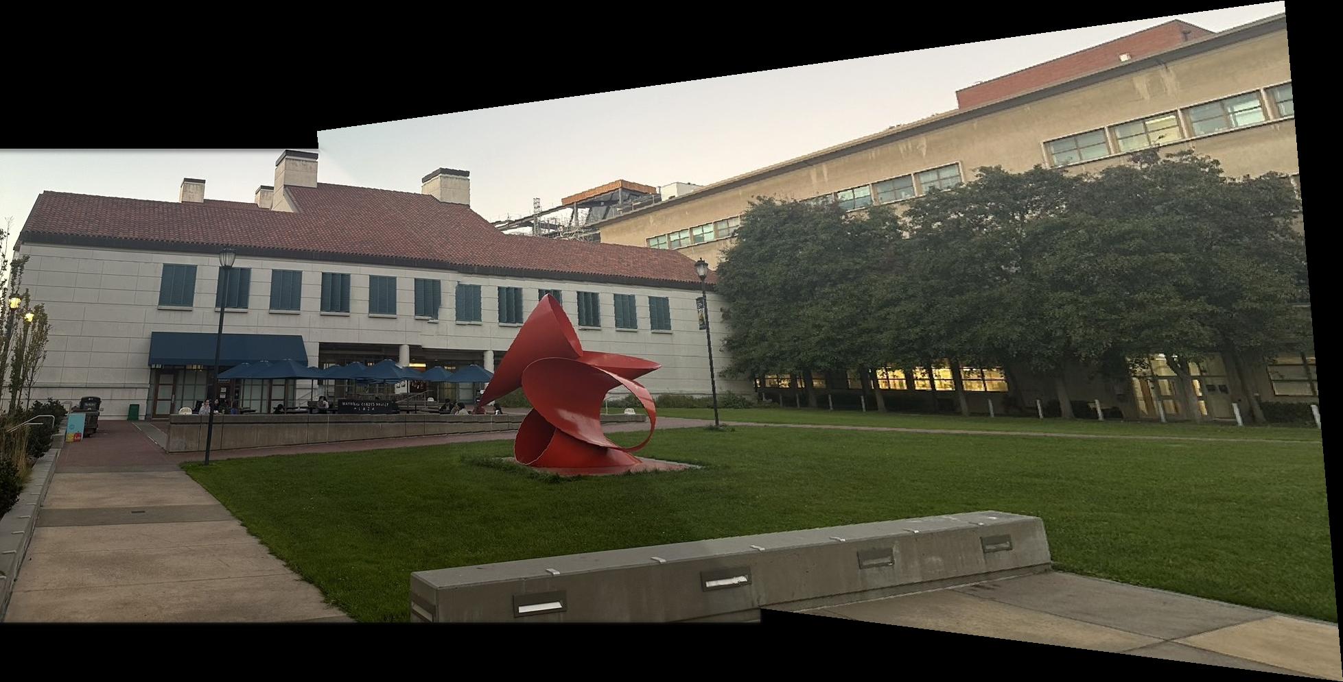
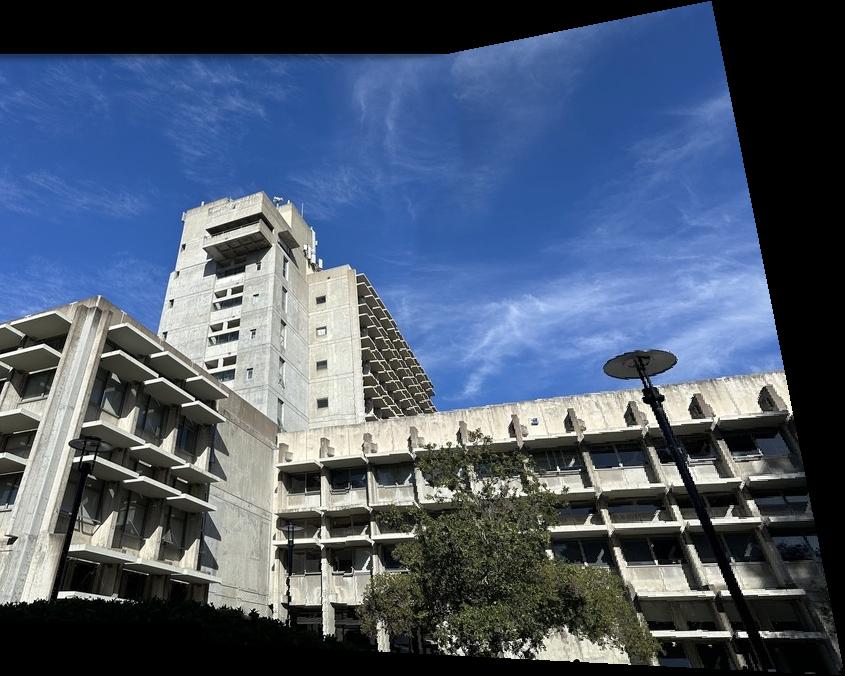
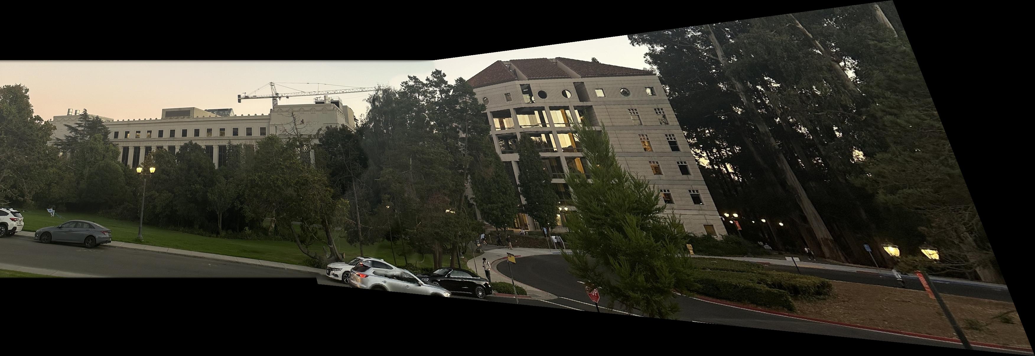
We then use the same method as the previous part of the project to get the final mosaic image. The image below shows the result of the Image Mosaic.




What have you learned ?
The thing I have learned from this project is how can I was able to use linear algebra to get the homography matrix and then use it to create the mosaic image which is a very interesting thing that we can do from a simple linear algebra.