Part 0: Setup
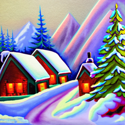
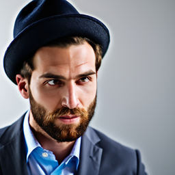
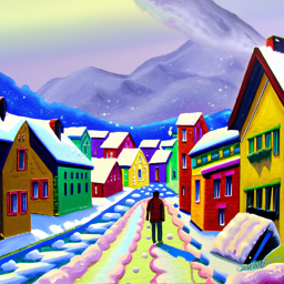
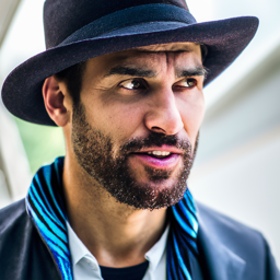
We start first with some setup where we are using the DeepFloyd IF diffusion model and we are showing the 3 text prompts and display the caption and the output of the model. We have that the first set of image has the number of inference steps are 20




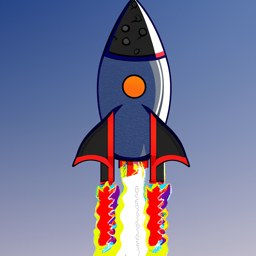


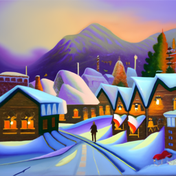
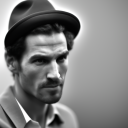
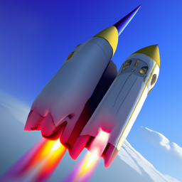
Part 1: Sampling Loops
1.1 Implementing the Forward Process
The first step I did is to write the forward process where we use the equation that was given to us sepcifically I use the following equation
\[ x_t = \sqrt{\bar{\alpha}_t} x_0 + \sqrt{1 - \bar{\alpha}_t} \epsilon \quad \text{where} \quad \epsilon \sim \mathcal{N}(0, 1) \]
which is essentially given a clean image \( x_0 \) we will get a noisy image \( x_t \) at time step \( t \) by sampling from a Gaussian noise with mean \( \sqrt{\bar{\alpha}_t} \) and variance \( \sqrt{1 - \bar{\alpha}_t} \). We implement the forward(im,t) function and the result below show the test image at noise level [0, 250, 500, 750]


1.2 Classical Denoising
Given now that we have the noisy images we want to try to denoise these images the first thing we can try is to use the Gaussian blur filtering (we used the kernel size to be 13 with sigma to be 2) to try to remove the noise the result below shows the result of applying gaussian blur at each time step [250, 500, 750]


As we can see from this that this is not looking good at all so we will try to use other method instead
1.3 One-Step Denoising
We will use the pretraiend diffusion model to denoise the image we can use this to recover the Gaussian noise from the image the image below show the result of the 3 noisy image at time step [250, 500, 750] and also the one-step denoised for each of the image


Again this look not the best however, it is still better than the gaussian blur earlier that we did now the next section we will do the iterative denoising
1.4 Iterative Denoising
Instead of doing one step denoising we can do a much better job by denoising each step and get the clear image at the end. To do this we first need to create a list of timesteps that we will call it as stided_timesteps where the first item in the list correspond to the noisiest image and then the last timesteps is the one that is a clean image so we used the stided_timesteps from T = 990 to T = 0 in steps of 30. Once we do that then for each of the timestep we use the following formula and we implement the function iterative_denois(image, i_start)
\[ x_t = \frac{\sqrt{\bar{\alpha}_t \beta_t}}{1 - \bar{\alpha}_t} x_0 + \frac{\sqrt{\alpha_t (1 - \bar{\alpha}_t)}}{1 - \bar{\alpha}_t} x_t + v_\sigma \]
Where:
- \( x_t \) is your image at timestep \( t \)
- \( x_{t'} \) is your noisy image at timestep \( t' \) where \( t' < t \) (less noisy)
- \( \bar{\alpha}_t \) is defined by
alphas_cumprod, as explained above. - \( \alpha_t = \frac{\bar{\alpha}_t}{\bar{\alpha}_{t'}} \)
- \( \beta_t = 1 - \alpha_t \)
- \( x_0 \) is our current estimate of the clean image using equation 2 just like in section 1.3
- \( v_\sigma \) is random noise, which in the case of DeepFloyd is also predicted.
We started first with i_start = 10 and the images below show the result of the noisy image of 5th loop of denoising and the final predicted clean image using iterative denoising, predicted clean image using single denoising step annd predicted clean image using gaussing bluring


1.5 Diffusion Model Sampling
Once we get everything working now we can started to do some sampling image completely from the noise that is we set the i_start to be 0 the images below some sample 5 images


1.6 Classifier-Free Guidance
One thing we note here is that the image generated is not very good so we have that we can do better by applying the classifier free guidance that is we compute the noise estimage of both a conditional and unconditional and then we denote the final noise as where \( \epsilon_{c} \) denote the epsilon noised estimated conditional and \( \epsilon_{u} \) denote the epsilon noised estimated unconditional
\[ \epsilon = \epsilon_{u} + \gamma (\epsilon_{c} - \epsilon_{u}) \]
We implemented the iterative denoise cfg function and using the scale factor of 7 and show the images of 5 sample the images are below


1.7 Image-to-Image Translation
From the previous part we have that we take a real image and we add noise to it and then denoise but this part we will try to take the original image noise a little bit and force it back onto the image manifold without any conditioning. We use the iterative_denoise_cfg function using a starting index of [1, 3, 5,7,10,20] steps and show the results


Editing Hand-Drawn and Web Image
Now we will try to use it to the web images and also the Hand-Drawn the images below show the result


1.7.2 Inpainting
We then apply the above proces such that we have an original image that is \( x_{orig} \) and a binary mask \( m \) then w can create a new image that has the same content whenever the mask is 0 and the new content whenever the mask is 1. This is done by using the normal diffusion step that we did however at every step we also have the following \[ x_t = mx_{t} + (1 - m)forward(x_{orgin},t) \] The images below show the result of the inpainting of the 3 images.


1.7.3 Text-Conditional Image-to-Image Translation
The next thing we can do is that instead of putting the text prompt of "a high quality photo" we can change our text prompt so that the image will generated from that text prompt and look similar to the original when we increase the noise level. The images below show the result where the first image we used the text prompt "a rocket ship", second image we used "robot head", and the third image we used "a strawberry".


1.8 Visual Anagrams
Now we can do something that is very cool that is we can use our diffusion model to make the visual anagrams that is when we look at the image we can see one thing and when we flipped the image then we will see another thing. This is done by the following method we will denoise image \( x_{t} \) at step \( t \) and then we use the first prompt to obtain the noise \( \epsilon_{1} \) and then we flip the \(x_{t} \) and use the second prompt to obtain the noise \( \epsilon_{2} \) and then we can flip \(\epsilon_{2}\) and then we can average the noise to get what we want. \[ \begin{align} \epsilon_{1} &= \text{UNet}(x_{t}, t, \text{prompt}_1) \\ \epsilon_{2} &= \text{flip}(\text{UNet}(\text{flip}(x_{t}), t, \text{prompt}_2)) \\ \epsilon &= \frac{\epsilon_{1} + \epsilon_{2}}{2} \end{align} \]


1.9 Hybrid Images
The last thing we can do is that we can create the hybrid images just like in project 2. In order to this we can do something that is very similar to the previous part that is we are doing the following \[ \begin{align} \epsilon_{1} &= \text{UNet}(x_{t}, t, \text{prompt}_1) \\ \epsilon_{2} &= \text{UNet}(x_{t}, t, \text{prompt}_2) \\ \epsilon &= f_{\text{lowpass}}(\epsilon_{1}) + f_{\text{highpass}}(\epsilon_{2}) \end{align}] where we have that that the we use the gaussian filter to get the low pass filter and high pass filter with kernel size of 33 and sigma of 2. The images below show some of the result of the hybrid images. We get the inspiration of the caption from here For the first set of images we use the following prompts "a lithograph of a skull" and "a lithograph of waterfalls", for the second set of images we use the following prompts "a lithograph of a pig" and "a lithograph of waterfalls", for the third set of images we use the following prompts "a lithograph of a panda" and "a lithograph of flowers".


Part B: Diffusion Models from Scratch!
1.2 Using the UNet to Train a Denoiser
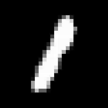
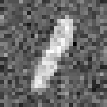
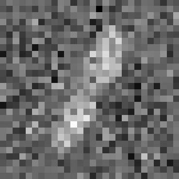
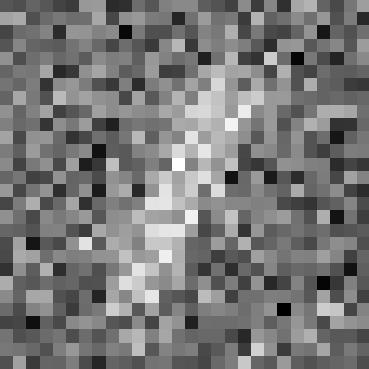
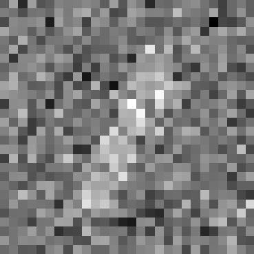
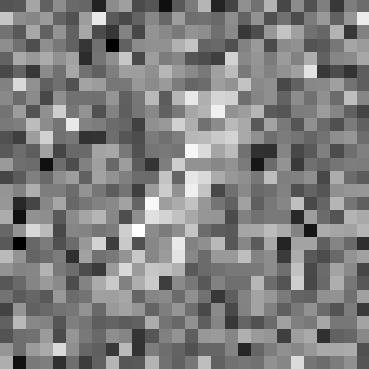
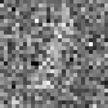
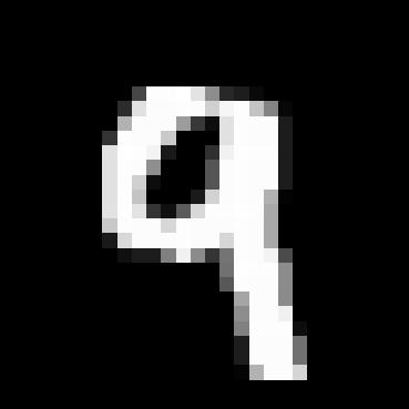
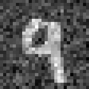
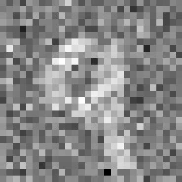
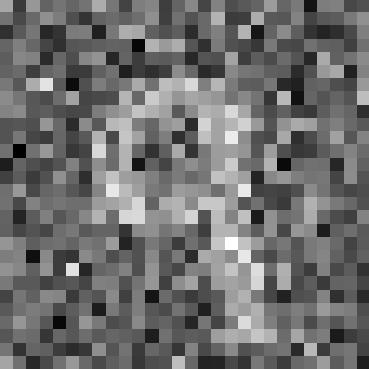
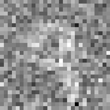
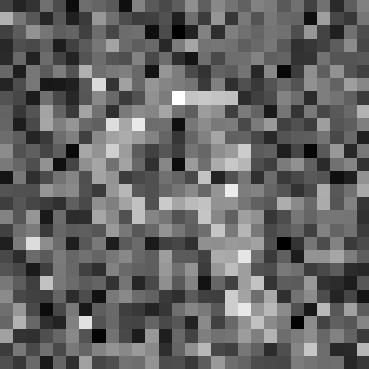
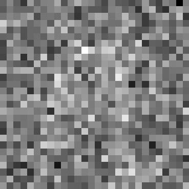
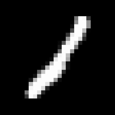
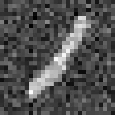
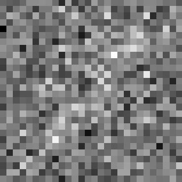
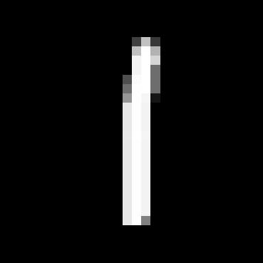
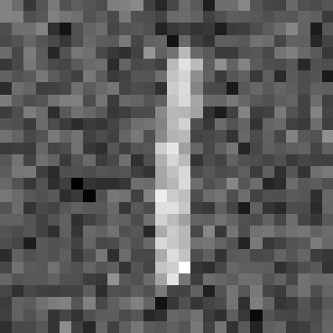
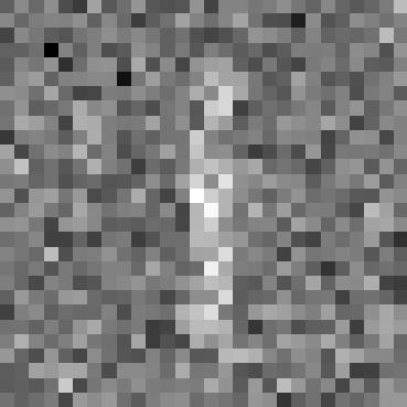
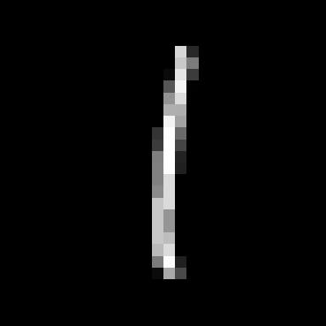
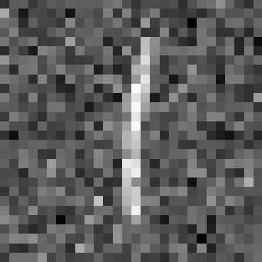
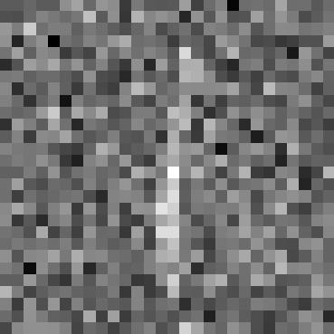
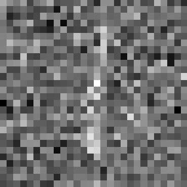
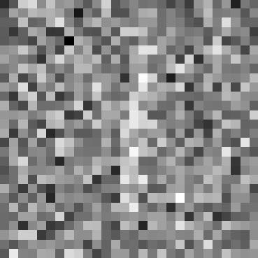
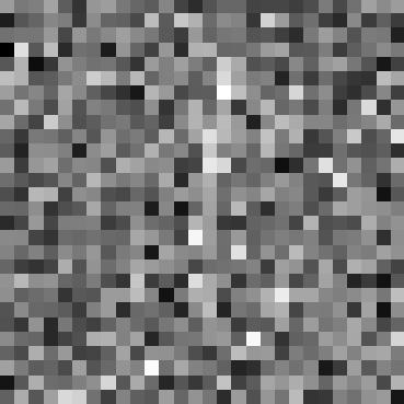
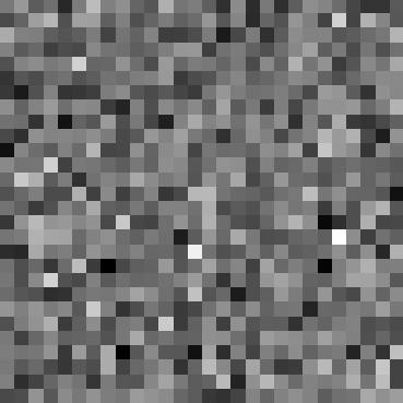
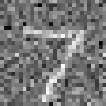
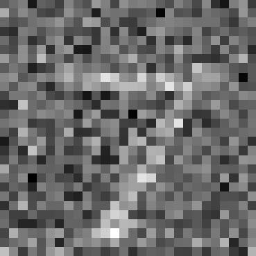
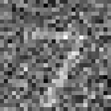
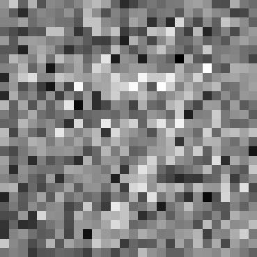
Now that we already have all the operations needed for implement UNet. We can use that to train a denoiser \(D_{\theta} \) such that it denoise the noisy image \(z \) and we want to get the clean image (\(x \)). We can do this by using the L2 loss and we have that \[ z = x + \sigma \epsilon, where \quad \epsilon \sim N(0,1) \] The images below the diferent denoising processes from \( \sigma = 0.0, 0.2, 0.4, 0.6, 0.8, 1.0 \).
1.2.1 Training
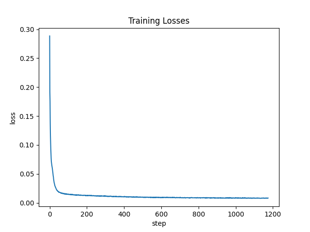
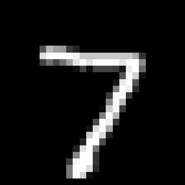
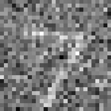
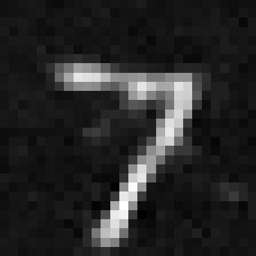
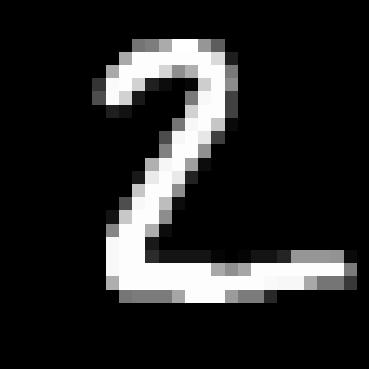
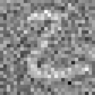
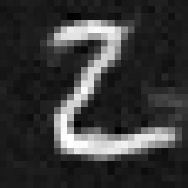
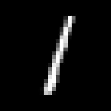
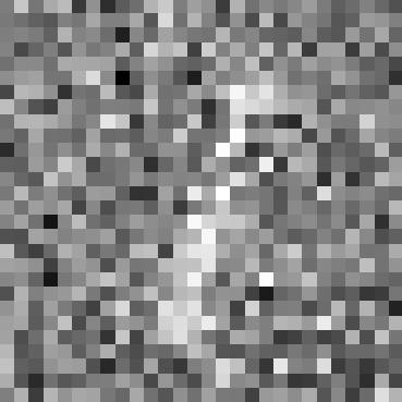
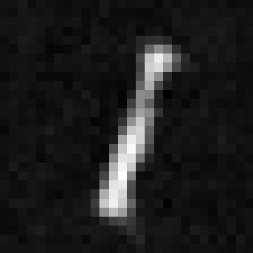
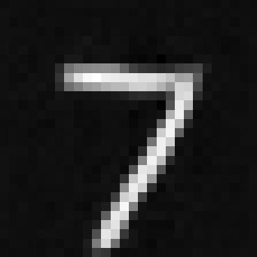
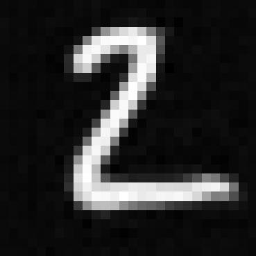
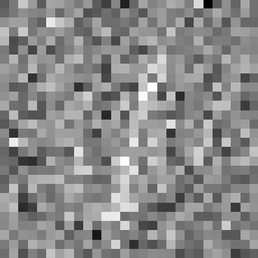
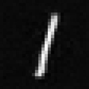
We then use the dataset and train our U-network for 5 epochs with the batch size of 256, hidden size of 128, and learning rate of 1e-4. We also use the sigma to be 0.5 and we shows the train losses for mini batch in every epoch so that is every batch size of 256. The images below show the training loss curve. We also show some sample of denosing at epoch 1 and epoch 5.



1.2.2 Out-of-Distribution Testing
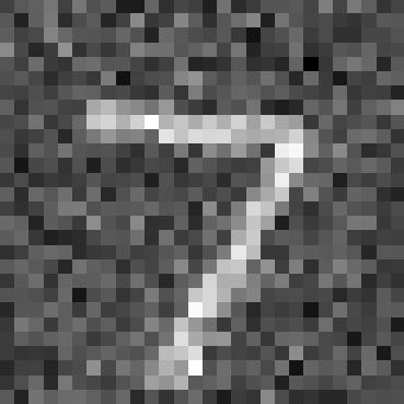
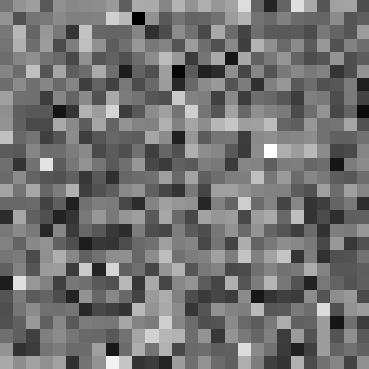
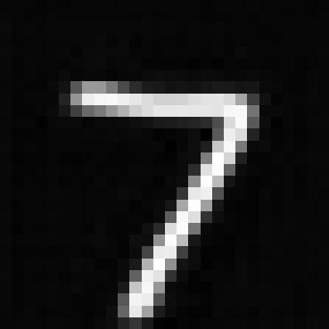
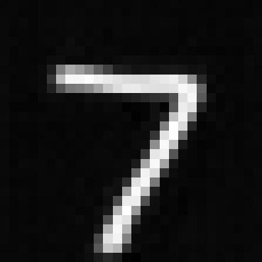
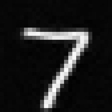
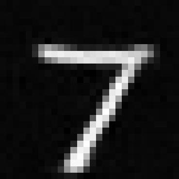
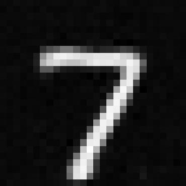
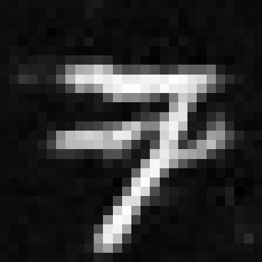
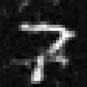
Once we are done with training we can use our model to do out-of-distribution testing. That is we used the trained model with noise 0.5 to denoise the images with noise level 0.0, 0.2, 0.4, 0.6, 0.8, 1.0.

Part 2
2.2 Training the UNet and 2.3 Sampling from the UNet
Once we defined the newly FCBlock and as we can see that the one step denoising might not be the best so w will try to implent to denoise the image iteratively the first thing we do is to add the time condition and use that to train our model. Since I finished this befroe the spec got change so my hyperparameter is the same as the previous part (that is batch size of 256, hidden size of 128, and learning rate of 1e-4) and also the loss present here is the train losses in every mini batch_size in every epoch that is every 256.
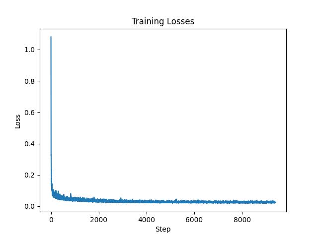
Epoch 1 sample time condition


Epoch 5 sample time condition


Epoch 10 sample time condition


Epoch 15 sample time condition


Epoch 20 sample time condition


2.4 Adding Class-Conditiong to UNet and 2.5 Sampling from the Class-Conditioned UNet
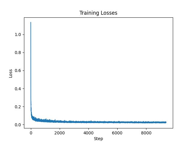
Epoch 1 sample class condition


Epoch 5 sample class condition


Epoch 10 sample class condition


Epoch 15 sample class condition


Epoch 20 sample class condition


